feec.polar.examples.poisson_2d

Solve manufactured 2D Poisson problems on polar mapped domains.

This file is not meant to be imported as a standard module, but rather run as a script, either serially or in parallel. The script builds analytical or spline-approximated disk-like domains (disk, target, or Czarny), assembles and solves the scalar Poisson system, applies optional treatments of the polar singularity (C0/C1 CONGA or C1 polar projectors), solves the resulting linear system, computes L2/H1 errors against the exact solution, and plots the result.

Typing python poisson_2d.py -h shows all the available command-line options. As an example, a parallel simulation with 6 MPI processes may be run with:

mpirun -n 6 python poisson_2d.py -S -d 3 3 -t disk -D 0.2 -m 'C0conga'

Functions

compute_errors(phi, phi_ref, M, S)	Compute relative L2 and H1 errors of a numerical solution.
parse_input_arguments()
plot_solution(use_spline_mapping, model, ...)	Plot exact solution, numerical solution and error.
run_poisson_2d(*, test_case, shift_D, R, ...)

Classes

CongaLaplacian(S, M, P, alpha)	Linear operator for the CONGA discretization of the Poisson problem.
ErrorDiagnostics(ref_l2, ref_h1, rel_l2, rel_h1)
Poisson2D(domain_log, mapping, phi_log, rho_log)	Exact solution to the 2D Poisson equation with Dirichlet boundary conditions, to be employed for the method of manufactured solutions.

Details

Solve manufactured 2D Poisson problems on polar mapped domains.

This file is not meant to be imported as a standard module, but rather run as a script, either serially or in parallel. The script builds analytical or spline-approximated disk-like domains (disk, target, or Czarny), assembles and solves the scalar Poisson system, applies optional treatments of the polar singularity (C0/C1 CONGA or C1 polar projectors), solves the resulting linear system, computes L2/H1 errors against the exact solution, and plots the result.

Typing python poisson_2d.py -h shows all the available command-line options. As an example, a parallel simulation with 6 MPI processes may be run with:

mpirun -n 6 python poisson_2d.py -S -d 3 3 -t disk -D 0.2 -m 'C0conga'

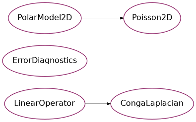
class Poisson2D(domain_log, mapping, phi_log, rho_log)

Bases: PolarModel2D

Exact solution to the 2D Poisson equation with Dirichlet boundary conditions, to be employed for the method of manufactured solutions.

\((\partial^2_{xx} + \partial^2_{yy}) \phi(x,y) = -\rho(x,y)\)

Parameters:

domain_logsympde.topology.Domain

Logical domain on which the solution is defined.

mappingsympde.topology.Mapping

Mapping from the logical domain to the physical domain.

phi_logsympy.Expr

Exact scalar potential in logical coordinates.

rho_logsympy.Expr

Source term in logical coordinates.

static disk(R, shift_D)

Solve Poisson’s equation on a disk of radius R centered at (x,y) = (0, 0), with logical coordinates (s, theta):

• The radial coordinate s belongs to the interval [0, R];

• The angular coordinate theta belongs to the interval [0, 2 * pi).

\(\phi(x,y) = (1 - ((x^2 + y^2) / R^2) ** 4) * sin(kx * x) * cos(ky * y)\).

Parameters:

Rfloat

Radius of the disk.

shift_Dfloat

Shafranov shift.

Returns:

Poisson2D

Poisson model containing the logical domain, mapping, exact solution and source term.

static target()

Solve Poisson’s equation on a polar domain, with logical coordinates (s, theta):

• The radial coordinate s belongs to the interval [0, 1];

• The angular coordinate theta belongs to the interval [0, 2 * pi).

The shape of the domain is set by parameter k in [0, 1): for k = 0 we have a disk and for k –> 1 the disk is horizontally squeezed.

The parameter D in (-(1 - k)/2, (1 - k)/2) moves horizontally the pole within the shape.

The parameter c1, c2 are just shifts on the plane of the domain.

\(\phi(x,y) = (1 - s^8)\sin(k_x(x - 0.5))\cos(k_y y)\).

static czarny()

Solve Poisson’s equation on a czarny domain, with logical coordinates (s, theta):

• The radial coordinate s belongs to the interval [0, 1];

• The angular coordinate theta belongs to the interval [0, 2 * pi).

\(\phi(x,y) = (1 - s^8)\sin(\pi x)\cos(\pi y)\).

property phi_log

property rho_log

property phi_log_callable

property rho_log_callable

class CongaLaplacian(S, M, P, alpha)

Bases: LinearOperator

Linear operator for the CONGA discretization of the Poisson problem.

Parameters:

SStencilMatrix

Stiffness matrix.

MStencilMatrix

Mass matrix.

P{C0PolarProjection_V0, C1PolarProjection_U0}

CONGA projection onto the conforming polar spline space.

alphafloat

Penalization parameter for CONGA methods.

Attributes:

SStencilMatrix

Stiffness matrix.

MStencilMatrix

Mass matrix.

P{C0PolarProjection_V0, C1PolarProjection_U0}

CONGA projection onto the conforming polar spline space.

alphafloat

Penalization parameter for CONGA methods.

W0StencilVectorSpace

Coefficient space on which the operator acts.

dot(x, out=None)

Apply the LinearOperator self to the Vector v.

The result is written to the Vector out, if provided.

Parameters:

vVector

The vector to which the linear operator (self) is applied. It must belong to the domain of self.

outVector

The vector in which the result of the operation is stored. It must belong to the codomain of self. If out is None, a new vector is created and returned.

Returns:

Vector

The result of the operation. If out is None, a new vector is returned. Otherwise, the result is stored in out and out is returned.

transpose(conjugate=False)

Transpose the LinearOperator .

If conjugate is True, return the Hermitian transpose.

tosparse()

Convert to a sparse matrix in any of the formats supported by scipy.sparse.

toarray()

Convert to Numpy 2D array.

property domain

The domain of the linear operator - an element of Vectorspace

property codomain

The codomain of the linear operator - an element of Vectorspace

property dtype

The data type of the coefficients of the linear operator, upon convertion to matrix.

class ErrorDiagnostics(ref_l2: float, ref_h1: float, rel_l2: float, rel_h1: float)

Bases: object

ref_l2: float

ref_h1: float

rel_l2: float

rel_h1: float

compute_errors(phi, phi_ref, M, S)

Compute relative L2 and H1 errors of a numerical solution.

Parameters:

phiFemField

Numerical solution.

phi_refFemField

Reference solution.

MStencilMatrix

Mass matrix used to compute the L2 norm.

SStencilMatrix

Stiffness matrix used to compute the H1 norm.

Returns:

ErrorDiagnostics

Reference L2 and H1 norms and relative L2 and H1 errors.

plot_solution(use_spline_mapping, model, ncells, periodic, V0_h, refine=10)

Plot exact solution, numerical solution and error.

Parameters:

use_spline_mappingbool

Whether a spline mapping is used.

modelPoisson2D

Poisson model containing the mapping and exact solution.

ncellssequence of int

Number of grid cells along each logical direction.

periodicsequence of bool

Periodicity along each logical direction.

V0_hTensorFemSpace

Discrete finite element space of the numerical solution.

refineint, default=10

Refinement factor for plotting.

run_poisson_2d(*, test_case, shift_D, R, ncells, degree, use_spline_mapping, smooth_method, alphaCONGA, tol, maxiter, verbose, mpi_comm)

parse_input_arguments()