feec.polar.examples.analytical_solutions

Analytical solutions for the 2D transverse-electric Maxwell problem in a disk.

We collect both time-harmonic solutions and initial conditions. Transverse- electric (TE) means that the electric field is a 1-form with two components \((E_x, E_y)\), while the magnetic field is a 2-form with a single component \(B_z\). We assume that a perfect electric conductor (PEC) is placed at the boundary of the domain.

This module can be run as a script to visualize the analytical solution of interest. The command line argument --solution allows switching between "cavity" and "gaussian".

Functions

main(solution_name)	Visualize an analytical solution of the 2D TE Maxwell problem.
parse_input_arguments()

Classes

CircularCavitySolution(R, c, m, n[, D, scale])	Time-harmonic solution of Maxwell's equations in a disk-like domain with perfectly conducting walls.
GaussianInitialCondition(sigma, x0, y0[, scale])	Initial Gaussian circular wave for the TE Maxwell test.
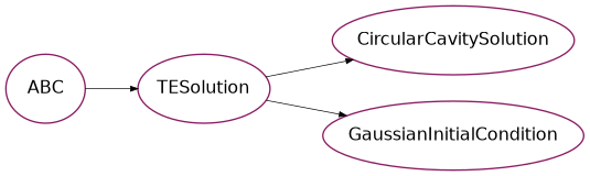
TESolution()	Base class for analytical/initial solutions of the 2D TE Maxwell problem.

Details

Analytical solutions for the 2D transverse-electric Maxwell problem in a disk.

We collect both time-harmonic solutions and initial conditions. Transverse- electric (TE) means that the electric field is a 1-form with two components \((E_x, E_y)\), while the magnetic field is a 2-form with a single component \(B_z\). We assume that a perfect electric conductor (PEC) is placed at the boundary of the domain.

This module can be run as a script to visualize the analytical solution of interest. The command line argument --solution allows switching between "cavity" and "gaussian".

class TESolution

Bases: ABC

Base class for analytical/initial solutions of the 2D TE Maxwell problem.

The physical fields are

E = (Ex, Ey), B = Bz.

Subclasses must provide the physical field components.

abstract Ex_ex(t, x, y)

abstract Ey_ex(t, x, y)

abstract Bz_ex(t, x, y)

class CircularCavitySolution(R, c, m, n, D=0, scale=1)

Bases: TESolution

Time-harmonic solution of Maxwell’s equations in a disk-like domain with perfectly conducting walls. This is a “transverse electric” solution, with E = (Ex, Ey) and B = Bz. The logical domain is [0, R] x [0, 2pi].

Parameters:

Rfloat

domain radius

cfloat

Speed of light in arbitrary units.

m, nint

Mode number. Warning: m > 0, n >= 0.

Dfloat, default=0.0

Shift of logical center (in “Target” mapping with c0=D*R2, c1=0, k=0, D=D).

scale: float, default=1.0

Rescaling the values by a real factor.

Es_ex(t, s, theta)

Et_ex(t, s, theta, s_factor=True)

if s_factor: multiply by s (as in logical field)

B_ex(t, s, theta, s_factor=True)

if s_factor: multiply by s (as in logical field)

dB_dt_ex(t, s, theta)

= dB/dt

get_radius_angle(x, y)

Ex_ex(t, x, y)

Ey_ex(t, x, y)

Bz_ex(t, x, y)

class GaussianInitialCondition(sigma, x0, y0, scale=1)

Bases: TESolution

Initial Gaussian circular wave for the TE Maxwell test.

This class defines the initial condition used for the Gaussian wave propagation experiment. It is not an exact time-dependent Maxwell solution. The electric field is initialized as a localized rotational Gaussian pulse,

E0(x, y) = scale * (y - y0, -(x - x0))

• exp(-((x - x0)^2 + (y - y0)^2) / (2 sigma^2)),

and the magnetic field is initialized as

B0 = curl E0 = d_x Ey - d_y Ex.

Parameters:

sigmafloat

Width of the Gaussian pulse (> 0).

x0, y0float

Center of the Gaussian pulse in physical coordinates.

scalefloat, default=1.0

Amplitude scaling factor for the initial fields.

Ex_ex(t, x, y)

Ey_ex(t, x, y)

Bz_ex(t, x, y)

Bz = curl E = d_x Ey - d_y Ex

dBz_dt_ex(t, x, y)

∂/∂t(Bz) = -curl(E)

main(solution_name)

Visualize an analytical solution of the 2D TE Maxwell problem. Plots the electric and magnetic fields in the physical domain and performs a consistency check of Faraday’s law.

Parameters:

solution_name{“cavity”, “gaussian”}

Name of the analytical solution to visualize.

parse_input_arguments()