B-splines FEM solver for Poisson equation (2D)#
In this section, we show hoa to use simplines to solve a 2D Poisson problem with homogeneous boundary conditions $$
\nabla^2 u = f, \Omega, \ u = 0, \partial \Omega $\( where the computation domain \)\Omega$ is the unit square.
# needed imports
from numpy import zeros, ones, linspace, zeros_like, asarray
import numpy as np
from matplotlib.pyplot import plot, show
import matplotlib.pyplot as plt

%matplotlib inline
from psydac.fem.splines import SplineSpace
from psydac.fem.tensor  import TensorFemSpace
from psydac.linalg.stencil import StencilMatrix
from psydac.linalg.stencil import StencilVector
from psydac.ddm.cart import DomainDecomposition
from gallery_section_04 import assemble_stiffness_2d
from gallery_section_04 import assemble_vector_2d
Create the Finite Elements Space#
In 2D, our Spline function space is defined as
which is basicaly $\( \mathcal{V}_h = \mathcal{V}_h^1 \otimes \mathcal{V}_h^2 \)\( where \)\( \mathcal{V}_h^1 := \texttt{span}\{ B_{i_1}^{p_1}, ~ 1 \le i_1 \le n_1\} \)\( and \)\( \mathcal{V}_h^2 := \texttt{span}\{ B_{i_2}^{p_2}, ~ 1 \le i_2 \le n_2\} \)$
# create the spline space for each direction
x1min = 0. ; x1max = 1.
nelements1 = 1
degree1 = 2
grid1 = np.linspace( x1min, x1max, num=nelements1+1 )
V1 = SplineSpace(degree=degree1, grid=grid1)

x2min = 0. ; x2max = 1.
nelements2 = 1
degree2 = 2
grid2 = np.linspace( x2min, x2max, num=nelements2+1 )
V2 = SplineSpace(degree=degree2, grid=grid2)
dd = DomainDecomposition(ncells=[V1.ncells, V2.ncells], periods=[False, False])
# create the tensor space
V = TensorFemSpace(dd, V1, V2)
Assemble the Stiffness Matrix#
The stiffness matrix entries are defined as
where $\( B_{\textbf{i}}(x_1,x_2) := B_{i_1}(x_1)B_{i_2}(x_2), \quad \textbf{i} := (i_1,i_2) \)\( and \)\( B_{\textbf{j}}(x_1,x_2) := B_{j_1}(x_1)B_{j_2}(x_2), \quad \textbf{j} := (j_1,j_2) \)$
stiffness = StencilMatrix(V.vector_space, V.vector_space)
stiffness = assemble_stiffness_2d( V, matrix=stiffness )
Assemble the rhs#
The right hand side entries are defined as
rhs = StencilVector(V.vector_space)

f = lambda x,y: 2*x*(1 - x) + 2*y*(1 - y)
rhs = assemble_vector_2d( f, V, rhs=rhs )
Imposing boundary conditions#
s1, s2 = V.vector_space.starts
e1, e2 = V.vector_space.ends

# ... needed for iterative solvers
# left  bc at x=0.
stiffness[s1,:,:,:] = 0.
rhs[s1,:]           = 0.
# right bc at x=1.
stiffness[e1,:,:,:] = 0.
rhs[e1,:]           = 0.
# lower bc at y=0.
stiffness[:,s2,:,:] = 0.
rhs[:,s2]           = 0.
# upper bc at y=1.
stiffness[:,e2,:,:] = 0.
rhs[:,e2]           = 0.
# ...

# ... needed for direct solvers
# boundary x = 0
#stiffness[s1,:,0,:] = 1.
# boundary x = 1
#stiffness[e1,:,0,:] = 1.
# boundary y = 0
#stiffness[:,s2,:,0] = 1.
# boundary y = 1
#stiffness[:,e2,:,0] = 1.
# ...
From now on, you can use the function apply_dirichlet to set the dirichlet boundary conditions for both the matrix and rhs.
# convert the stencil matrix to scipy sparse
stiffness = stiffness.tosparse()


```python
# convert the stencil vector to a nd_array
rhs = rhs.toarray()
#from scipy.sparse import csc_matrix, linalg as sla

#lu = sla.splu(csc_matrix(stiffness))
#x = lu.solve(rhs)
from scipy.sparse.linalg import cg
x, info = cg( stiffness, rhs, rtol=1e-7, maxiter=100 )
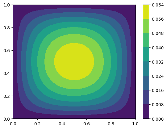
from utilities.plot import plot_field_2d
nbasis  = [W.nbasis for W in V.spaces]
knots   = [W.knots for W in V.spaces]
degrees = [W.degree for W in V.spaces]
u = x.reshape(nbasis)
plot_field_2d(knots, degrees, u) ; plt.colorbar()