B-Splines#
Given a subdivision \(\{x_0 < x_1 < \cdots < x_r\}\) of the interval \(I = [x_0, x_r]\), the \textbf{Schoenberg space} is the space of piecewise polynomials of degree \(p\), on the interval \(I\) and given regularities \(\{k_1, k_2, \cdots, k_{r-1}\}\) at the internal points \(\{x_1, x_2, \cdots, x_{r-1}\}\).
Given \(m\) and \(p\) as natural numbers, let us consider a sequence of non decreasing real numbers \(T=\{t_i\}_{0\leqslant i \leqslant m}\). \(T\) is called knots sequence. From a knots sequence, we can generate a B-splines family using the reccurence formula \ref{eq:bspline-reccurence}.
Definition 4 (B-Splines using Cox-DeBoor Formula)
The j-th B-spline of degree \(p\) is defined by the recurrence relation:
where
for \(0 \leq j \leq m-p-1\).
Remark 4
When working with Bernstein polynomials, we introduced the convention \(B_i^n=0\) for all \(i<0\) or \(i>n\). For B-Splines, we have a similar convetion \(N_j^p=0\) if \(j<0\) or \(j>n\). In addition, we also assume \(\frac{0}{0} = 0\), when using the formula \ref{eq:bspline-reccurence} and \(N_j^0 = 0\) if \(t_j = t_{j+1}\).
# needed imports
import numpy as np
from numpy import empty
import matplotlib.pyplot as plt
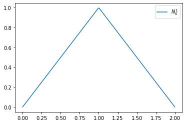
Example 8
We consider a linear B-Spline with the knot vector \(T = [0, 1, 2]\)
def N1_0(t):
    if t >= 0 and t< 1: return t
    if t >= 1 and t< 2: return 2-t
    return 0.

xs = np.linspace(0., 2., 200)
plt.plot(xs, [N1_0(x) for x in xs], label='$N_0^1$')
plt.legend()
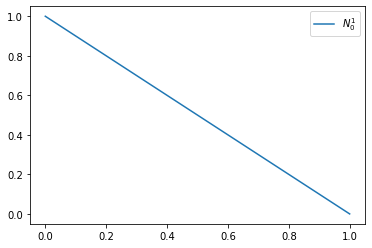
Example 9
We consider a linear B-Spline with the knot vector \(T = [0, 0, 1]\)
def N1_0(t):
    if t >= 0 and t< 1: return 1-t
    return 0.

xs = np.linspace(0., 1., 200)
plt.plot(xs, [N1_0(x) for x in xs], label='$N_0^1$')
plt.legend()
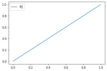
Example 10
We consider a linear B-Spline with the knot vector \(T = [0, 1, 1]\)
def N1_0(t):
    if t >= 0 and t< 1: return t
    return 0.

xs = np.linspace(0., 1., 201)[:-1]
plt.plot(xs, [N1_0(x) for x in xs], label='$N_0^1$')
plt.legend()
Example 11
We consider linear B-Splines with the knot vector \(T = [0, 0, 1, 1]\)
def N1_0(t):
    if t >= 0 and t< 1: return 1-t
    return 0.

def N1_1(t):
    if t >= 0 and t< 1: return t
    return 0.

xs = np.linspace(0., 1., 201)[:-1]
plt.plot(xs, [N1_0(x) for x in xs], label='$N_0^1$')
plt.plot(xs, [N1_1(x) for x in xs], label='$N_1^1$')
plt.legend()
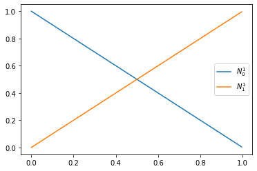
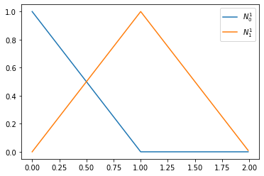
Example 12
We consider linear B-Splines with the knot vector \(T = [0, 0, 1, 2]\)
def N1_0(t):
    if t >= 0 and t< 1: return 1-t
    return 0.

def N1_1(t):
    if t >= 0 and t< 1: return t
    if t >= 1 and t< 2: return 2-t
    return 0.

xs = np.linspace(0., 2., 201)[:-1]
plt.plot(xs, [N1_0(x) for x in xs], label='$N_0^1$')
plt.plot(xs, [N1_1(x) for x in xs], label='$N_1^1$')
plt.legend()
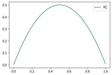
Example 13
We consider a quadratic B-Spline with the knot vector \(T = [0, 0, 1, 1]\)
def N2_0(t):
    if t >= 0 and t< 1: return 2*t*(1-t)
    return 0.

xs = np.linspace(0., 1., 201)[:-1]
plt.plot(xs, [N2_0(x) for x in xs], label='$N_0^2$')
plt.legend()
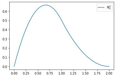
Example 14
We consider a quadratic B-Spline with the knot vector \(T = [0, 0, 1, 2]\)
T = [0, 0, 1, 2]
def N2_0(t):
    if t >= 0 and t< 1: return 2*t-3./2.*t**2
    if t >= 1 and t< 2: return 0.5*(2-t)**2
    return 0.

xs = np.linspace(0., 2., 200)
plt.plot(xs, [N2_0(x) for x in xs], label='$N_0^2$')
plt.legend()
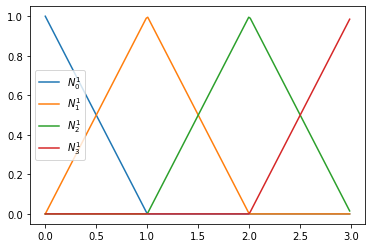
Example 15
We consider linear B-Splines with the knot vector \(T = [0, 0, 1, 2, 3, 3]\)
def N1_0(t):
    if t >= 0 and t< 1: return 1-t
    return 0.

def N1_1(t):
    if t >= 0 and t< 1: return t
    if t >= 1 and t< 2: return 2-t
    return 0.

def N1_2(t):
    if t >= 1 and t< 2: return t-1
    if t >= 2 and t< 3: return 3-t
    return 0.

def N1_3(t):
    if t >= 2 and t< 3: return t-2
    return 0.


xs = np.linspace(0., 3., 201)[:-1]
plt.plot(xs, [N1_0(x) for x in xs], label='$N_0^1$')
plt.plot(xs, [N1_1(x) for x in xs], label='$N_1^1$')
plt.plot(xs, [N1_2(x) for x in xs], label='$N_2^1$')
plt.plot(xs, [N1_3(x) for x in xs], label='$N_3^1$')
plt.legend()
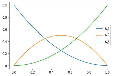
Example 16
We consider quadratic B-Splines with the knot vector \(T = [0, 0, 0, 1, 1, 1]\)
def N2_0(t):
    if t >= 0 and t< 1: return (1-t)**2
    return 0.

def N2_1(t):
    if t >= 0 and t< 1: return 2*t*(1-t)
    return 0.

def N2_2(t):
    if t >= 0 and t< 1: return t**2
    return 0.

xs = np.linspace(0., 1., 201)[:-1]
plt.plot(xs, [N2_0(x) for x in xs], label='$N_0^2$')
plt.plot(xs, [N2_1(x) for x in xs], label='$N_1^2$')
plt.plot(xs, [N2_2(x) for x in xs], label='$N_2^2$')
plt.legend()
B-Splines properties#
B-Splines have many interesting properties that are listed below. In general, most of the proofs are done by induction on the B-Spline degree.
Proposition 7
B-splines are piecewise polynomial of degree \(p\)
Remark 5
The B-splines functions associated to open knots sequences without internal knots, \textit{i.e.} the length of the knots sequence is exactly \(2p+2\), are the Bernstein polynomials of degree\(p\).
Proposition 8 (compact support)
\(N_j^p(t) = 0\) for all \(t \notin [t_j, t_{j+p+1})\).
Proposition 9
\label{prop:non-vanishing-bsplines} If \(t \in~ [ t_j,t_{j+1} ) \), then only the \textit{B-splines} \(\{ N_{j-p}^p,\cdots,N_{j}^p \}\) are non vanishing at \(t\).
Proposition 10 (non-negativity)
\(N_j^p(t) \ge 0, \quad \forall t \in [ t_j, t_{j+p+1} ) \)
Proposition 11 (Partition of unity)
\(\sum N_i^{p}(t) = 1, \forall t \in \mathbb{R}\)
Remark 6
The previous sum \(\sum N_i^{p}(t)\) has a meaning since for every \(t \in \mathbb{R}\), only \(p+1\) B-Splines are non-vanishing.
Remark 7
For the sake of simplicity, we shall avoid using summation indices on linear expansion of B-Splines.
Lemma 1
Proposition 12 (Marsden’s idenity)
where
Thanks to Marsden’s identity and the proposition \ref{prop:non-vanishing-bsplines}, we now are able to prove the local linear independence of the B-Splines basis functions.
Proposition 13 (Local linear independence)
On each interval \([t_j, t_{j+1})\), the B-Splines are lineary independent.
Remark 8
We will see in the Approximation theory part, that the B-Splines family has also a global linear independence property.
Proposition 14 (Derivatives of B-Splines)
The derivative of B-Splines can be computed reccursivly by deriving the formula \ref{eq:bspline-reccurence}, which gives
Evaluation of B-Splines#
Given a knot sequence \(T=\{t_i\}_{0\leqslant i \leqslant n + p}\), we are interested in the algorithmic evaluation of B-Splines of degree \(p\).
Warning
Add evaluation diagram
For a given real point \(x\), it is done in two steps:
find the knot span index \(j\), such that \(x \in~ ] t_j,t_{j+1} [ \)
evaluate all non-vanishing B-Splines \(N_{j-p}^p, \cdots, N_j^p\)
The first point is achieved by the function implemented by the following function:
def find_span( knots, degree, x ):
    # Knot index at left/right boundary
    low  = degree
    high = 0
    high = len(knots)-1-degree

    # Check if point is exactly on left/right boundary, or outside domain
    if x <= knots[low ]: returnVal = low
    elif x >= knots[high]: returnVal = high-1
    else:
        # Perform binary search
        span = (low+high)//2
        while x < knots[span] or x >= knots[span+1]:
            if x < knots[span]:
                high = span
            else:
                low  = span
            span = (low+high)//2
        returnVal = span

    return returnVal
The second point is implemented by the following function, that returns all non-vanishing B-Splines at \(x\)
def all_bsplines( knots, degree, x, span ):
    left   = empty( degree  , dtype=float )
    right  = empty( degree  , dtype=float )
    values = empty( degree+1, dtype=float )

    values[0] = 1.0
    for j in range(0,degree):
        left [j] = x - knots[span-j]
        right[j] = knots[span+1+j] - x
        saved    = 0.0
        for r in range(0,j+1):
            temp      = values[r] / (right[r] + left[j-r])
            values[r] = saved + right[r] * temp
            saved     = left[j-r] * temp
        values[j+1] = saved

    return values
The following function plots all B-Splines given a knot vector and a polynomial degree.
def plot_splines(knots, degree, nx=100):
    xmin = knots[degree]
    xmax = knots[-degree-1]

    # grid points for evaluation
    xs = np.linspace(xmin,xmax,nx)

    # this is the number of the BSplines in the Schoenberg space
    N = len(knots) - degree - 1

    ys = np.zeros((N,nx), dtype=np.double)
    for ix,x in enumerate(xs):
        span = find_span( knots, degree, x )
        b    = all_bsplines( knots, degree, x, span )
        ys[span-degree:span+1, ix] = b[:]

    for i in range(0,N):
        plt.plot(xs,ys[i,:], label='$N_{}$'.format(i+1))
    plt.legend(loc=9, ncol=4)
Knots vector families#
There are two kind of knots vectors, called clamped and unclamped. Both families contains uniform and non-uniform sequences.
The following are examples of such knots vectors
Clamped knots (open knots vector)#
uniform#
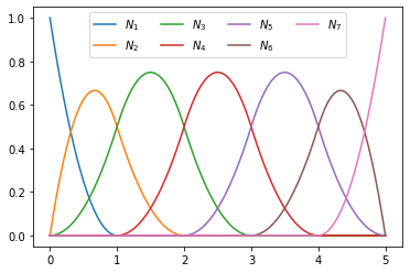
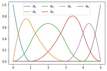
Example 17
T = np.array([0, 0, 0, 1, 2, 3, 4, 5, 5, 5])

plot_splines(T, degree=2, nx=100)
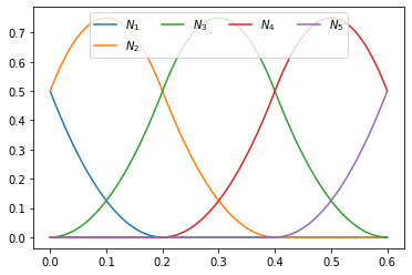
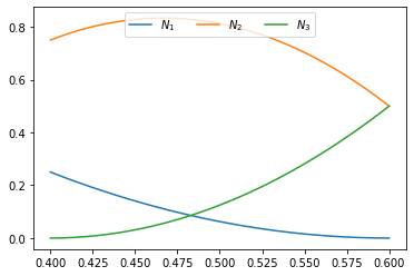
Example 18
T = [-0.2, -0.2, 0.0, 0.2, 0.4, 0.6, 0.8, 0.8]

plot_splines(T, degree=2, nx=100)
non-uniform#
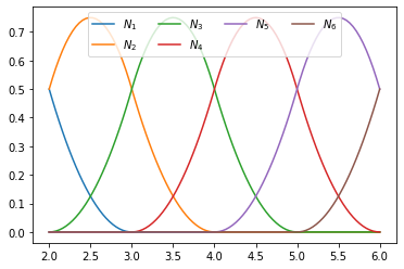
Example 19
T = [0, 0, 0, 1, 3, 4, 5, 5, 5]

plot_splines(T, degree=2, nx=100)
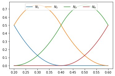
Example 20
T = [-0.2, -0.2, 0.4, 0.6, 0.8, 0.8]

plot_splines(T, degree=2, nx=100)
Unclamped knots#
uniform#
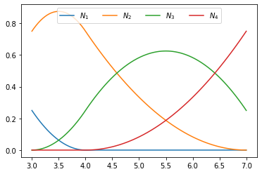
Example 21
T = [0, 1, 2, 3, 4, 5, 6, 7, 8]

plot_splines(T, degree=2, nx=100)
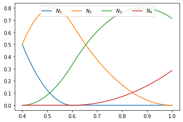
Example 22
T = [-0.2, 0.0, 0.2, 0.4, 0.6, 0.8, 1.0]

plot_splines(T, degree=2, nx=100)
non-uniform#
Example 23
T = [0, 0, 3, 4, 7, 8, 9]

plot_splines(T, degree=2, nx=100)
Example 24
T = [-0.2, 0.2, 0.4, 0.6, 1.0, 2.0, 2.5]

plot_splines(T, degree=2, nx=100)