Bézier curves

We recall the definition of a Bézier curve:

\[ \begin{align} \mathcal{C}(t) = \sum_{k=0}^n \mathbf{P}_k B_k^n(t) \end{align} \]

where \(\left( \mathbf{P} \right)_{0 \le k \le n}\) are the control points or Bézier points.

Evaluation of a point on Bézier curve

The following function evaluates a Bézier curve, given the control points \(P\) at \(x\). The degree of the Bernstein polynomials is computed from the length of \(P\).

def point_on_bezier_curve(P,x):
    n = len(P) - 1
    b = all_bernstein(n, x)
    c = 0.
    for k in range(0, n+1):
        c += b[k]*P[k]
    return c

Examples

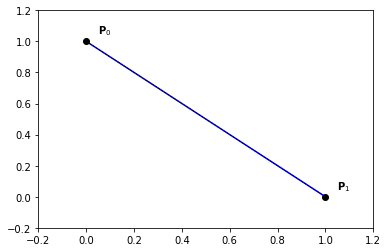
Example 1

nt = 200
ts = np.linspace(0., 1., nt)

P = np.zeros((2, 2))
P[:, 0] = [0., 1.]
P[:, 1] = [1., 0.]

Q = np.zeros((nt, 2))
for i,t in enumerate(ts):
    Q[i,:] = point_on_bezier_curve(P,t)

plt.plot(Q[:,0], Q[:,1], '-b')
plt.plot(P[:,0], P[:,1], '--ok', linewidth=0.7)

for i in range(0, 2):
    x,y = P[i,:]
    plt.text(x+0.05,y+0.05,'$\mathbf{P}_{' + str(i) + '}$')

plt.axis([-0.2, 1.2, -0.2, 1.2])

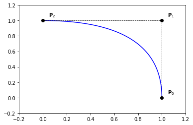
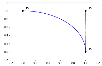
Example 2

nt = 200
ts = np.linspace(0., 1., nt)

P = np.zeros((3, 2))
P[:, 0] = [1., 1., 0.]
P[:, 1] = [0., 1., 1.]

Q = np.zeros((nt, 2))
for i,t in enumerate(ts):
    Q[i,:] = point_on_bezier_curve(P,t)

plt.plot(Q[:,0], Q[:,1], '-b')
plt.plot(P[:,0], P[:,1], '--ok', linewidth=0.7)

for i in range(0, 3):
    x,y = P[i,:]
    plt.text(x+0.05,y+0.05,'$\mathbf{P}_{' + str(i) + '}$')

plt.axis([-0.2, 1.2, -0.2, 1.2])

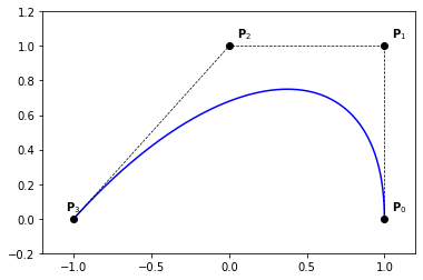
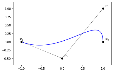
Example 3

nt = 200
ts = np.linspace(0., 1., nt)

P = np.zeros((4, 2))
P[:, 0] = [1., 1., 0., -1.]
P[:, 1] = [0., 1., 1.,  0.]

Q = np.zeros((nt, 2))
for i,t in enumerate(ts):
    Q[i,:] = point_on_bezier_curve(P,t)

plt.plot(Q[:,0], Q[:,1], '-b')
plt.plot(P[:,0], P[:,1], '--ok', linewidth=0.7)

for i in range(0, 3):
    x,y = P[i,:]
    plt.text(x+0.05,y+0.05,'$\mathbf{P}_{' + str(i) + '}$')
i = 3
x,y = P[i,:]
plt.text(x-0.05,y+0.05,'$\mathbf{P}_{' + str(i) + '}$')

plt.axis([-1.2, 1.2, -0.2, 1.2])

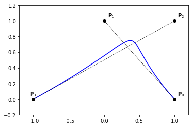
Example 4

nt = 200
ts = np.linspace(0., 1., nt)

P = np.zeros((4, 2))
P[:, 0] = [1., 1.,  0., -1.]
P[:, 1] = [0., 1., -0.5,  0.]

Q = np.zeros((nt, 2))
for i,t in enumerate(ts):
    Q[i,:] = point_on_bezier_curve(P,t)

plt.plot(Q[:,0], Q[:,1], '-b')
plt.plot(P[:,0], P[:,1], '--ok', linewidth=0.7)

for i in range(0, 3):
    x,y = P[i,:]
    plt.text(x+0.05,y+0.05,'$\mathbf{P}_{' + str(i) + '}$')
i = 3
x,y = P[i,:]
plt.text(x-0.05,y+0.05,'$\mathbf{P}_{' + str(i) + '}$')

plt.axis([-1.2, 1.2, -0.7, 1.2])

Example 5

nt = 200
ts = np.linspace(0., 1., nt)

P = np.zeros((4, 2))
P[:, 0] = [1., 0., 1., -1.]
P[:, 1] = [0., 1., 1.,  0.]

Q = np.zeros((nt, 2))
for i,t in enumerate(ts):
    Q[i,:] = point_on_bezier_curve(P,t)

plt.plot(Q[:,0], Q[:,1], '-b')
plt.plot(P[:,0], P[:,1], '--ok', linewidth=0.7)

for i in range(0, 3):
    x,y = P[i,:]
    plt.text(x+0.05,y+0.05,'$\mathbf{P}_{' + str(i) + '}$')
i = 3
x,y = P[i,:]
plt.text(x-0.05,y+0.05,'$\mathbf{P}_{' + str(i) + '}$')

plt.axis([-1.2, 1.2, -0.2, 1.2])

Derivatives of a Bezier curve

Using the formulae \ref{eq:bernstein-der}, we have

\[ \begin{align} \mathcal{C}^\prime(t) = \sum_{k=0}^n \mathbf{P}_k {B_k^n}^\prime(t) = \sum_{k=0}^n n \mathbf{P}_k \left(B_{k-1}^{n-1}(x) - B_k^{n-1}(x) \right) \end{align} \]

by reordering the indices, we get \ref{eq:bezier-curve-der}

\[ \begin{align} \mathcal{C}^\prime(t) &= \sum_{k=0}^{n-1} n \left( \mathbf{P}_{k+1} - \mathbf{P}_k \right) B_k^{n-1}(t) \label{eq:bezier-curve-der} \end{align} \]

Therefor, we get the direct acces to the first order derivatives at the extremeties of a Bézier curve using the formulae \ref{eq:bezier-curve-der-1-ext}

\[\begin{split} \begin{align} \begin{cases} \mathcal{C}^\prime(0) = n \left( \mathbf{P}_{1} - \mathbf{P}_0 \right) \\ \mathcal{C}^\prime(1) = n \left( \mathbf{P}_{n} - \mathbf{P}_{n-1} \right) \end{cases} \label{eq:bezier-curve-der-1-ext} \end{align} \end{split}\]

Second derivatives can also be computed directly from the control points using the formulae \ref{eq:bezier-curve-der-2-ext}

\[\begin{split} \begin{align} \begin{cases} \mathcal{C}^{\prime\prime}(0) = n(n-1) \left( \mathbf{P}_{0} - 2 \mathbf{P}_1 + \mathbf{P}_{2} \right) \\ \mathcal{C}^{\prime\prime}(1) = n(n-1) \left( \mathbf{P}_{n} - 2 \mathbf{P}_{n-1} + \mathbf{P}_{n-2} \right) \end{cases} \label{eq:bezier-curve-der-2-ext} \end{align} \end{split}\]

Definition 2 (\(r^{th}\) forward difference)

Let us consider a set of (control) points \(\mathbf{P}\). The \(r^{th}\) forward difference of \(\mathbf{P}\) is defined as
$\( \begin{align} \triangle^r \mathbf{P}_i := \triangle^{r-1} \mathbf{P}_{i+1} - \triangle^{r-1} \mathbf{P}_i \end{align} \)\( with \)\( \begin{align} \triangle \mathbf{P}_i = \triangle^1 \mathbf{P}_i := \mathbf{P}_{i+1} - \mathbf{P}_i \end{align} \)$

Proposition 2 (High order dirivatives)

\[ \begin{align} \mathcal{C}^{(r)}(t) = \frac{n!}{\left( n-r \right)!} \sum\limits_{i=0}^{n-r} \triangle^r \mathbf{P}_i B_i^{n-r}(t) \label{eq:bezier-high-deriv} \end{align} \]

Eqs (\ref{eq:bezier-curve-der-1-ext}) and (\ref{eq:bezier-curve-der-2-ext}) can be generelaized for high order derivatives. We have in fact the following result:

Remark 1

The derivatives of a Bézier curve at its extremeties up to order \(r\) depend only on the first (or last) \(r+1\) control points, and vice versa.

Proposition 3

\label{prop:bezier-forward-difference} $\(\triangle^r \mathbf{P}_0 = \sum\limits_{i=0}^{r} \left( -1 \right)^{r-i} \binom{r}{i} \mathbf{P}_i \)$

Integration of Bezier curves

Proposition 4

A primitive of A Bézier curve \(\mathcal{C}(t) = \sum_{k=0}^n \mathbf{P}_k B_k^n(t)\) has the Bézier representation

\[ \begin{align} \left( \int \mathcal{C} \right) (t) = \sum_{k=0}^{n+1} \mathbf{Q}_k B_k^{n+1}(t) \label{eq:bezier-primitive} \end{align} \]

where

\[ \begin{align} \mathbf{Q}_k := \mathbf{Q}_{k-1} + \frac{1}{n+1} \mathbf{P}_{k-1} = \mathbf{Q}_{0} + \frac{1}{n+1} \left( \sum\limits_{i=0}^{k-1} \mathbf{P}_{i} \right) \end{align} \]

Here, \(\mathbf{Q}_{0}\) denotes an arbitrary integration constant.

Remark 2

Using Eq. (\ref{eq:bezier-primitive}), we have \(\int_0^1 \mathcal{C}(t)~dt = \frac{1}{n+1}\left( \sum\limits_{i=0}^n \mathbf{P}_i \right)\).

Properties of Bezier curves

Because of the symmetry of the Bernstein polynomials, we have

• \(\sum_{k=0}^n \mathbf{P}_k B_k^n = \sum_{k=0}^n \mathbf{P}_k B_{n-k}^n\)

Thanks to the interpolation property, for \(B_0^n\) and \(B_n^n\), of the Bernstein polynomials at the endpoints, we get

• \(\mathcal{C}(0) = \mathbf{P}_0\) and \(\mathcal{C}(1) = \mathbf{P}_n\)

Using the partition unity property of the Bernstein polynomials, we get

• any point \(\mathcal{C}(t)\) is an affine combination of the control points

Therefor,

• Bézier curves are affinely invariant; i.e. the image curve \(\Phi(\sum_{k=0}^n \mathbf{P}_k B_k^n)\) of a Bézier curve, by an affine mapping \(\Phi\), is the Bézier curve having \(\left( \Phi(\mathbf{P}_i) \right)_{0 \le i \le n}\) as control points.

due to the partition unity of the Bernstein polynomials and their non-negativity,

• any point \(\mathcal{C}(t)\) is a convex combination of the control points

finally, we get the convex hull property,

• A Bézier curve lies in the convex hull of its control points

DeCasteljau Algorithm

In this section, we introduce the deCasteljau algorithm Algo. (\ref{algo:decasteljau}). The basic idea comes from the following remark; using the reccurence formulae Eq. (\ref{eq:bernstein-rec}), we have

\[\begin{split} \begin{align} \mathcal{C}(t) &= \sum_{k=0}^n \mathbf{P}_k B_k^n(t) = \sum_{k=0}^n \mathbf{P}_k \left( (1-t) B_k^{n-1}(t) + t B_{k-1}^{n-1}(t) \right) \\ &= \sum_{k=0}^{n-1} \mathbf{P}_k^1 B_k^{n-1}(t) \quad\quad\quad\quad\quad [\mathbf{P}_k^{1} := (1-t)\mathbf{P}_k + t \mathbf{P}_{k+1}] \\ &= \sum_{k=0}^{n-2} \mathbf{P}_k^2 B_k^{n-2}(t) \quad\quad\quad\quad\quad [\mathbf{P}_k^{2} := (1-t)\mathbf{P}_k^1 + t \mathbf{P}_{k+1}^1] \\ &= \ldots \\ &= \sum_{k=0}^{0} \mathbf{P}_k^n B_k^{0}(t) \quad\quad\quad\quad\quad [\mathbf{P}_k^{n} := (1-t)\mathbf{P}_k^{n-1} + t \mathbf{P}_{k+1}^{n-1}] \\ &= \mathbf{P}_0^n \end{align} \end{split}\]

Algorithm 1 (Evaluation of a Bézier curve, defined by its control points \(\mathbf{P}\) at \(x\))

Input \(\mathbf{P}, x\) Output \(value\)

\(n \gets { len } \left( \mathbf{P} \right) - 1\)

\(\mathbf{Q} \gets \mathbf{P}\)

For \(j \gets 0\) : \(n\)

For \(i \gets 0\) : \(n-j\)

$Q[i] \gets (1-x) Q[i] + x Q[i+1]$

Return \(Q[0]\)

def decasteljau(P, x):
    n = len(P) - 1
    Q = P.copy()
    x1 = 1.-x
    for j in range(1, n+1):
        for i in range(0, n-j+1):
            Q[i] = x1*Q[i] + x*Q[i+1]
    c = Q[0]
    return c

Conversion from monomial form

Let us consider a monomial representation of a curve

\[ \begin{align} \mathcal{C}(t) = \sum_{k=0}^n \mathbf{Q}_k t^k \end{align} \]

Since

\[\begin{split} \begin{align} t^k &= \frac{1}{\binom{n}{k}} \binom{n}{k} t^k \left(1-t+t \right)^{n-k} = \frac{1}{\binom{n}{k}} \left( \sum\limits_{i=0}^{n-k} \binom{n}{k} \binom{n-k}{n-k-i} t^{i+k} \left( 1-t \right)^{n-k-i} \right) \\ &= \frac{1}{\binom{n}{k}} \left( \sum\limits_{i=0}^{n-k} \binom{k+i}{k} B_{k+i}^n(t) \right) = \frac{1}{\binom{n}{k}} \left( \sum\limits_{j=0}^{n} \binom{j}{k} B_{j}^n(t) \right) \end{align} \end{split}\]

we get,

\[ \begin{align} \mathcal{C}(t) = \sum_{k=0}^n \mathbf{Q}_k t^k = \sum_{k=0}^n \mathbf{Q}_k \frac{1}{\binom{n}{k}} \left( \sum\limits_{j=0}^{n} \binom{j}{k} B_{j}^n(t) \right) \end{align} \]

hence,

\[ \begin{align} \mathcal{C}(t) = \sum_{j=0}^n \left(\sum\limits_{k=0}^{n} \frac{\binom{j}{k}}{\binom{n}{k}} \mathbf{Q}_k \right) B_{j}^n(t) \end{align} \]

which is a Bézier curve of the form

\[ \begin{align} \mathcal{C}(t) = \sum_{k=0}^n \mathbf{P}_k B_k^n(t) \end{align} \]

with

\[ \begin{align} \mathbf{P}_k = \sum\limits_{k=0}^{n} \frac{\binom{j}{k}}{\binom{n}{k}} \mathbf{Q}_k \end{align} \]

Remark 3

If \(\mathbf{Q}_k = 0\) for all \(k \geq 2\), then the control points are given by \(\mathbf{P}_k = \mathbf{Q}_0 + k \mathbf{Q}_1\).

Proposition 5 (Linear Precision)

Conversly, if the \(n+1\) control points \(\mathbf{P}\) lie equidistantly on a line, then \(\mathcal{C}\) is a linear polynomial, which can be written as \(\mathcal{C}(t) = \left(1-t\right) \mathbf{P}_0 + t \mathbf{P}_n\).

Conversion to monomial form

Given a Bézier curve \(\mathcal{C}(t) = \sum_{k=0}^n \mathbf{P}_k B_k^n(t)\), we can derive its monomial representation using the Taylor expansion,

\[\begin{split} \begin{align} \mathcal{C}(t) &= \sum\limits_{k=0}^n \frac{1}{k!}\mathcal{C}^{(k)}(0) t^k \\ &= \sum\limits_{k=0}^n \binom{n}{k} \triangle^k \mathbf{P}_0 t^k \end{align} \end{split}\]

Rational Bézier curves

We first introduce the notion of Rational Bernstein polynomials defined as, and \(w_i > 0, \forall i \in \left[0, n \right]\)

\[ \begin{align} R_k^n(t) := \frac{w_i B_k^n(t)}{\sum_{i=0}^n w_i B_i^n(t)} \label{eq:rational-bernstein} \end{align} \]

Proposition 6 (Properties of Rational Bernstein polynomials)

• \(R_k^n(x) \ge 0\), for all \(k \in \left[0, n \right]\) and \(x \in \left[ 0, 1 \right]\) \hfill [positivity]

• \(\sum_{k=0}^n R_k^n(x) = 1\), for all \(x \in \left[ 0, 1 \right]\) \hfill [partition of unity]

• \(R_0^n(0) = R_n^n(1) = 1\)

• \(R_k^n\) has exactly one maximum on the interval \(\left[ 0, 1 \right]\),

• Bernstein polynomials are Rational Bernstein polynomials when all weights are equal

Definition 3 (Rational Bézier curve)

\[ \begin{align} \mathcal{C}(t) = \sum_{k=0}^n \mathbf{P}_k R_k^n(t) \label{eq:bezier-curve} \end{align} \]

where \(R_k^n(t) := \frac{w_i B_k^n(t)}{\sum_{i=0}^n w_i B_i^n(t)}\) and \(w_i > 0, \forall i \in \left[0, n \right]\)

Example

Example 6

nt = 200
ts = np.linspace(0., 1., nt)

P = np.zeros((3, 2))
P[:, 0] = [1., 1., 0.]
P[:, 1] = [0., 1., 1.]

# weights
W = np.asarray([1., 1., 2.])

# weithed control points in 3D
Pw = np.zeros((3,3))
for i in range(0, 3):
    Pw[i,:2] = W[i]*P[i,:]
    Pw[i,2]  = W[i]

Qw = np.zeros((nt, 3))
for i,t in enumerate(ts):
    Qw[i,:] = point_on_bezier_curve(Pw,t)

Q = np.zeros((nt, 2))
Q[:,0] = Qw[:,0]/Qw[:,2]
Q[:,1] = Qw[:,1]/Qw[:,2]

plt.plot(Q[:,0], Q[:,1], '-b')
plt.plot(P[:,0], P[:,1], '--ok', linewidth=0.7)

for i in range(0, 3):
    x,y = P[i,:]
    plt.text(x+0.05,y+0.05,'$\mathbf{P}_{' + str(i) + '}$')

plt.axis([-0.2, 1.2, -0.2, 1.2])

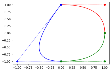
Composite Bézier curve

Example 7

n = 2

nt = 200
ts = np.linspace(0., 1., nt)

# ...
P = np.zeros((3, 2))
P[:, 0] = [1., 1., 0.]
P[:, 1] = [0., 1., 1.]

Q = np.zeros((nt, 2))
for i,t in enumerate(ts):
    Q[i,:] = point_on_bezier_curve(P,t)

plt.plot(Q[:,0], Q[:,1], '-r')
plt.plot(P[:,0], P[:,1], '--or', linewidth=0.7)
# ...

# ...
P = np.zeros((3, 2))
P[:, 0] = [0., -1., 0.]
P[:, 1] = [1., -1., -1.]

Q = np.zeros((nt, 2))
for i,t in enumerate(ts):
    Q[i,:] = point_on_bezier_curve(P,t)

plt.plot(Q[:,0], Q[:,1], '-b')
plt.plot(P[:,0], P[:,1], '--ob', linewidth=0.7)
# ...

# ...
P = np.zeros((3, 2))
P[:, 0] = [1., 1., 0.]
P[:, 1] = [0., -1., -1.]

Q = np.zeros((nt, 2))
for i,t in enumerate(ts):
    Q[i,:] = point_on_bezier_curve(P,t)

plt.plot(Q[:,0], Q[:,1], '-g')
plt.plot(P[:,0], P[:,1], '--og', linewidth=0.7)
# ...