3D example with VTK and ParaView

In this notebook we show how to solve a 3D problem in parallel, save the solution in HDF5 format and export it to VTK.

We solve the regularized curl-curl problem in 3D with a callable function for the source. In practice, the source could be the interpolation of some experimental data. Besides, we impose periodic boundary conditions everywhere in the boundary.

Let \(\Omega=[0, 10] \times [-2\pi, 2\pi]\times [-3, 1]\). We want to find \(u\in H(\mathrm{curl}, \Omega)\) such that

\[\mathrm{curl} \mathrm{curl} u + \mu u = f,\]

where \(\mu = \pi\), and \(f\) is a callable function (of the domain coordinates) for which we may not have a symbolic expression.

Since \(\mu>0\) the resulting operator is positive definite and we can use conjugate gradient to solve the system. In the case of the time-harmonic Maxwell problem we have that \(\mu<0\), which yields an indefinite operator and conjugate gradient is no longer guaranteed to converge.

Only for illustration here we use the callable function

\[f(x,y,z) = (10e^{-0.5(x-4)^2 - 1.5z^2 - 0.1y^2}, 0, \cos(y)\sin(\pi x / 5)),\]

and project it from \(H(\mathrm{curl}, \Omega)\) to the corresponding discretized space. This process is analogous with any callable vectorial function.

Step 1 : define the domain and spaces and discretize them

This is similar to what is done in other examples

import numpy as np
from mpi4py                     import MPI
from sympde.topology            import Cube
from sympde.topology            import VectorFunctionSpace
from psydac.api.discretization  import discretize

comm = MPI.COMM_WORLD # MPI communicator

Omega = Cube('Omega', bounds1=(0, 10), bounds2=(-2*np.pi, 2*np.pi), bounds3=(-3, 1)) # 3D cubic domain

W = VectorFunctionSpace('W', Omega, kind='hcurl') # Hcurl space

ncells = [25, 30, 11] # number of cells in each direction
degree = [3, 2, 2] # B-spline degree in each direction

periodic = [True, True, True] # set periodic BC in every direction

Omega_h = discretize(Omega, ncells=ncells, periodic=periodic, comm=comm)
Wh = discretize(W, Omega_h, degree=degree)

Step 2 : compute the matrix

We assemble the mass and curl curl matrices.

from sympde.topology      import elements_of, element_of
from sympde.expr.expr     import BilinearForm, LinearForm, integral
from sympde.calculus      import dot, curl
from psydac.api.settings  import PSYDAC_BACKENDS
from psydac.fem.basic     import FemField

backend_language = 'pyccel-gcc'
backend = PSYDAC_BACKENDS[backend_language]

u, v = elements_of(W, names='u, v') #trial and test functions

m = BilinearForm((u, v), integral(Omega, dot(u, v)))
mh = discretize(m, Omega_h, [Wh, Wh], backend=backend)
M = mh.assemble()  # Mass matrix

k = BilinearForm((u, v), integral(Omega, dot(curl(u), curl(v))))
kh = discretize(k, Omega_h, [Wh, Wh], backend=backend)
K = kh.assemble()  # Curl curl matrix

mu = np.pi

A = K + mu*M # system matrix, positive-definite

Step 3 : compute the right-hand size

We project a callable function to the vector space and use it to assemble the right-hand side of the system.

from psydac.feec.global_geometric_projectors    import GlobalGeometricProjectorHcurl
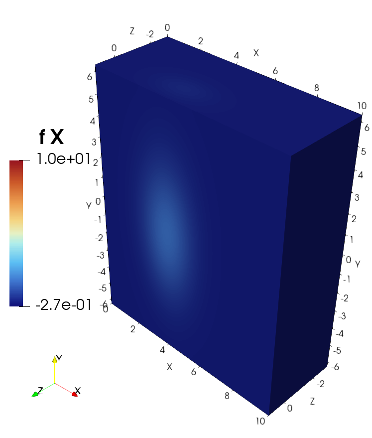
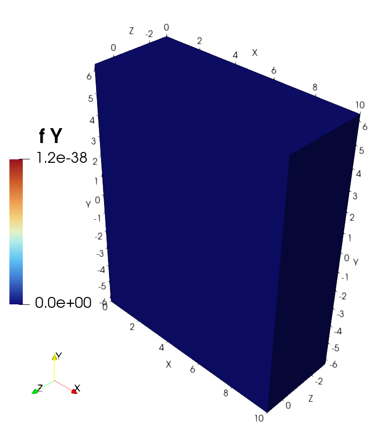
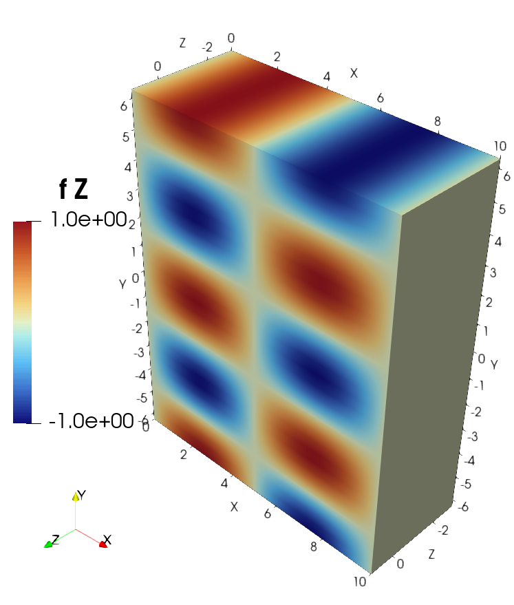
f_callable = [lambda x, y, z: 10*np.exp(-0.5*(x-4)**2 - 1.5*z**2 - 1e-1*y**2),
              lambda x, y, z: 0,
              lambda x, y, z: np.cos(y)*np.sin(x*np.pi/5)]

proj_Wh = GlobalGeometricProjectorHcurl(Wh, nquads=[p+1 for p in degree]) # get Hcurl projector, nquads is the number of points for the Gauss quadrature.
fh = proj_Wh(f_callable) # project callable to field in Wh

f = element_of(W, name='f') # free variable for the FemField

l = LinearForm(v, integral(Omega, dot(f,v)))
lh = discretize(l, Omega_h, Wh, backend=backend)
rhs = lh.assemble(f=fh)  # assmble RHS, f is a free parameter

Step 4 : solve the system

Solve the system using Conjugate Gradient. Notice that since \(\mu>0\), the matrix is positive definite.

from psydac.linalg.solvers import inverse

inv_A = inverse(A, solver='cg', tol=1e-2, maxiter=100) # invert using Conjugate Gradient

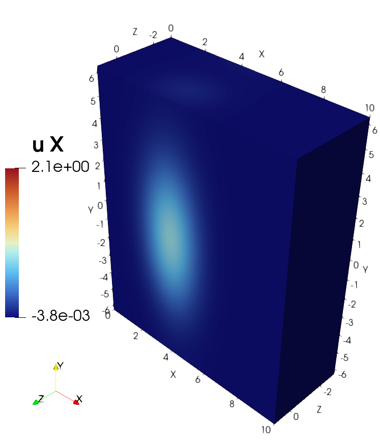
u = inv_A @ rhs # array of coefficients

uh = FemField(Wh, coeffs=u) # finite element field, callable

Step 5 : Save results to HDF5 format

We save the coefficients of the solution and the field used in the right-hand size. This step generates a YAML file containing the space information, and a HDF5 file that stores the coefficients. The fields are saved in parallel. This step does not include an evaluation of the fields on a grid.

# Save the results using OutputManager
from psydac.api.postprocessing import OutputManager
import os

os.makedirs('results_regularized_curlcurl', exist_ok=True)

Om = OutputManager(
    f'results_regularized_curlcurl/space_info_{Omega.name}.yml',
    f'results_regularized_curlcurl/field_info_{Omega.name}.h5',
    comm=comm,
    save_mpi_rank=True,
    mode = 'w'
)

Om.add_spaces(V=Wh)
Om.export_space_info()

Om.set_static() # the fields do not depend on time

save_fields = {
    'u': uh,
    'f': fh
}

Om.export_fields(**save_fields) # saves the coefficients of the fields

Om.close()

# This generates a YAML file containing the space information, and a HDF5 file that stores the solution coefficients.
# At this point the solution has not been evaluated on any grid.

Step 6 : Evaluate fields on a grid and export to VTK

Evaluate the saved fields on a grid and export the result to VTK format.

# Export the results to VTK using PostProcessManager
from psydac.api.postprocessing import PostProcessManager

Pm = PostProcessManager(
    domain=Omega,
    space_file=f'results_regularized_curlcurl/space_info_{Omega.name}.yml',
    fields_file=f'results_regularized_curlcurl/field_info_{Omega.name}.h5',
    comm=comm
)

Pm.export_to_vtk(
    f'results_regularized_curlcurl/visu_{Omega.name}',
    grid=None,
    npts_per_cell=[4,2,4],
    fields=save_fields.keys() # evaluate all the fields that were saved
)

Pm.close()
# If this file is run in sequential, then this step will generate a single .vtu file that can be opened with ParaView.
# If it is run in parallel, it generates a .vtu file per process (containing the local grid) and a .pvtu file. To visualize it in ParaView, open the .pvtu file.

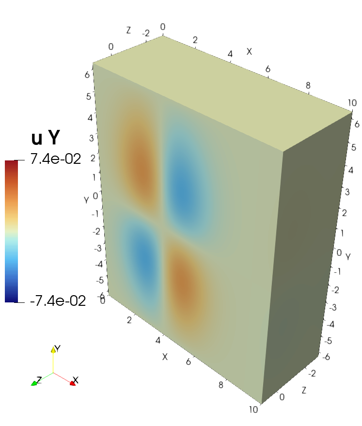
Visualization of the solution in ParaView

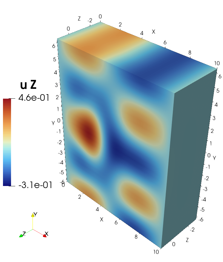
Visualization of the source in ParaView