
Example of solving the curl-curl eigenvalue problem#
In this notebook we show how to compute approximate eigenvalues for the curl-curl eigenvalue problem using the FEEC (Finite Element Exterior Calculus) API of PSYDAC. The problem reads as follows:
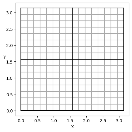
Let \(\Omega=[0, \pi] \times [0, \pi]\). We want to find \(\lambda >0\) and \(\boldsymbol{E} \in H_0(\mathrm{curl}, \Omega)\) such that
Step 1 : Building the domain#
This is similar to what is done in other examples. We leave the option to use a single patch or multiple patches. The FEEC interface is compatible with both.
[1]:
import numpy as np

single_patch = False

# degree of the splines in each direction
degree = (3, 3)

if single_patch:
    #number of cells in each direction
    ncells = [10, 10]

    from sympde.topology import Square, IdentityMapping
    logical_domain = Square('Omega', bounds1=(0, np.pi), bounds2=(0, np.pi))
    mapping = IdentityMapping('M1', dim=2)
    domain = mapping(logical_domain)

else:
    # We can give the shape of the multipatch domain
    # through the shape of the array containing the number of cells in each direction
    ncells = np.array([[5, 5],
                        [5, 5]])
    # The multipatch domain then has the following structure:
    # A | B
    # -----
    # C | D

    from psydac.feec.multipatch_domain_utilities import build_cartesian_multipatch_domain
    domain = build_cartesian_multipatch_domain(ncells, (0, np.pi), (0, np.pi), mapping='identity')

    # We now need to convert the ncells array into a dictionary,
    # where the keys are the patches
    ncells = {patch.name: [ncells[int(patch.name[2])][int(patch.name[4])],
            ncells[int(patch.name[2])][int(patch.name[4])]] for patch in domain.interior}


from sympde.utilities.utils import plot_domain
plot_domain(domain, isolines=True)
Step 2: Create and discretize the de Rham complex#
[2]:
from psydac.api.discretization import discretize
from sympde.topology import Derham

domain_h = discretize(domain, ncells=ncells)

derham = Derham(domain, ["H1", "Hcurl", "L2"])
derham_h = discretize(derham, domain_h, degree=degree)

V0h, V1h, V2h = derham_h.spaces
Step 3: Use the FEEC interface to get the operators#
The (broken) FEEC operators are given by: The conforming projections \(P^\ell: V^\ell_\mathrm{pw} \rightarrow V^\ell_h\), mapping from broken to continuous spaces. The broken derivatives \(D^\ell: V^\ell_\mathrm{pw} \rightarrow V^{\ell + 1}_\mathrm{pw}\) and the Hodge-operators \(H^\ell\) which can be seen as mass matrices.
[3]:
# conforming projectors with homogeneous boundary conditions
# (In  the single patch case, they only involve the zero BCs)
cP0, cP1, cP2 = derham_h.conforming_projectors(kind='linop', hom_bc = True)

# broken (patch-wise) derivative operators
bD0, bD1 = derham_h.derivatives(kind='linop')

# broken Hodge operators (mass matrices) and their inverses
H0, H1, H2 = derham_h.hodge_operators(kind='linop')
dH0, dH1, dH2 = derham_h.hodge_operators(kind='linop', dual=True)

from psydac.linalg.basic import IdentityOperator
I1 = IdentityOperator(V1h.coeff_space)
Step 4: Set up the system matrices#
The \(\mathrm{curl}\) operators are discretized by the conforming curl operator \(D^1 P^1\) and its transpose. The right-hand-side is given by the conforming mass matrix \((P^1)^T H^1 P^1\) where we also have to add a penalization term corresponding to the discontinuous jumps in the broken spaces: \((I - P^1)^T H^1 (I - P^1)\). In total, the discrete equation reads:
[4]:
CC = cP1.T @ bD1.T @ H2 @ bD1 @ cP1
RHS = cP1.T @ H1 @ cP1 + (I1 - cP1).T @ H1 @ (I1 - cP1)
Step 5: Scipy eigenvalue solver#
[5]:
def get_eigenvalues(nb_eigs, sigma, A_m, M_m):
    """
    Compute the eigenvalues of the matrix A close to sigma and right-hand-side M

    Parameters
    ----------
    nb_eigs : int
        Number of eigenvalues to compute
    sigma : float
        Value close to which the eigenvalues are computed
    A_m : sparse matrix
        Matrix A
    M_m : sparse matrix
        Matrix M
    """

    from scipy.sparse.linalg    import spilu, lgmres
    from scipy.sparse.linalg    import LinearOperator, eigsh, minres
    from scipy.linalg           import norm

    print('-----  -----  -----  -----  -----  -----  -----  -----  -----  -----  -----  -----  -----  -----  -----  ----- ')
    print(
        'computing {0} eigenvalues (and eigenvectors) close to sigma={1} with scipy.sparse.eigsh...'.format(
            nb_eigs,
            sigma))
    mode = 'normal'
    which = 'LM'
    # from eigsh docstring:
    #   ncv = number of Lanczos vectors generated ncv must be greater than k and smaller than n;
    #   it is recommended that ncv > 2*k. Default: min(n, max(2*k + 1, 20))
    ncv = 4 * nb_eigs
    try_lgmres = True
    max_shape_splu = 24000   # OK for nc=20, deg=6 on pretzel_f
    if A_m.shape[0] < max_shape_splu:
        print('(via sparse LU decomposition)')
        OPinv = None
        tol_eigsh = 0
    else:

        OP_m = A_m - sigma * M_m
        tol_eigsh = 1e-7
        if try_lgmres:
            print(
                '(via SPILU-preconditioned LGMRES iterative solver for A_m - sigma*M1_m)')
            OP_spilu = spilu(OP_m, fill_factor=15, drop_tol=5e-5)
            preconditioner = LinearOperator(
                OP_m.shape, lambda x: OP_spilu.solve(x))
            tol = tol_eigsh
            OPinv = LinearOperator(
                matvec=lambda v: lgmres(OP_m, v, x0=None, tol=tol, atol=tol, M=preconditioner,
                                        callback=lambda x: print(
                                            'cg -- residual = ', norm(OP_m.dot(x) - v))
                                        )[0],
                shape=M_m.shape,
                dtype=M_m.dtype
            )

        else:
            # from https://docs.scipy.org/doc/scipy/reference/generated/scipy.sparse.linalg.eigsh.html:
            # the user can supply the matrix or operator OPinv, which gives x = OPinv @ b = [A - sigma * M]^-1 @ b.
            # > here, minres: MINimum RESidual iteration to solve Ax=b
            # suggested in https://github.com/scipy/scipy/issues/4170
            print('(with minres iterative solver for A_m - sigma*M1_m)')
            OPinv = LinearOperator(
                matvec=lambda v: minres(
                    OP_m,
                    v,
                    tol=1e-10)[0],
                shape=M_m.shape,
                dtype=M_m.dtype)

    eigenvalues, eigenvectors = eigsh(
        A_m, k=nb_eigs, M=M_m, sigma=sigma, mode=mode, which=which, ncv=ncv, tol=tol_eigsh, OPinv=OPinv)

    print("done: eigenvalues found: " + repr(eigenvalues))
    return eigenvalues, eigenvectors
Step 6: Solve the system#
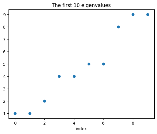
We solve for the first nb_eigs many eigenvalue closest to the reference value sigma. In the case nb_eigs=10 and sigma=5, the exact eigenvalues are the first 10 sum of squares, i.e. ref_sigmas = [1, 1, 2, 4, 4, 5, 5, 8, 9, 9].
[6]:
ref_sigmas = [
            1, 1,
            2,
            4, 4,
            5, 5,
            8,
            9, 9,
        ]
sigma = 5
nb_eigs = 10

eigenvalues, eigenvectors_transp = get_eigenvalues(nb_eigs, sigma, CC.tosparse(), RHS.tosparse())
-----  -----  -----  -----  -----  -----  -----  -----  -----  -----  -----  -----  -----  -----  -----  -----
computing 10 eigenvalues (and eigenvectors) close to sigma=5 with scipy.sparse.eigsh...
(via sparse LU decomposition)
done: eigenvalues found: array([1.00000003, 1.00000003, 2.00000006, 4.00000956, 4.00000956,
       5.00000959, 5.00000959, 8.00001912, 9.00025536, 9.00025536])
Step 7: Plot the eigenvalues#
[7]:
import matplotlib.pyplot as plt

fig,ax = plt.subplots(1,1)
ax.set_title(f"The first {nb_eigs} eigenvalues")
im = ax.scatter(np.arange(eigenvalues.size), eigenvalues)
plt.xlabel('index');
Testing the notebook#
[8]:
import ipytest
ipytest.autoconfig(raise_on_error=True)
[9]:
%%ipytest

l2_error = np.sqrt(np.sum((eigenvalues - ref_sigmas)**2))

def test_l2error():
    assert l2_error < 5e-04
.                                                                                            [100%]
1 passed in 0.01s