Solving Helmholtz’s equation on non-periodic topological domains

In this notebook, we will show how to solve Helmholtz’s equation on single patch and multipatch domains. As we are running this in a notebook, everything will be run in serial and hence we are limiting ourselves to a fairly coarse discretization to avoid taking too much time. However, PSYDAC allows for hybrid MPI + OpenMP parallelization with barely any changed to the code. The lines that are impacted by that will be preceeded by their MPI equivalent

Step 1 : Building the domain

PSYDAC uses the powerful topological tools of SymPDE to build a large variety of domains. Here we show how to create a Square.

import numpy as np

from sympde.topology import Square
Omega=Square()

Step 2: Defining the Abstract PDE model using SymPDE

from sympde.calculus import grad, dot
from sympde.calculus import minus, plus

from sympde.expr.expr          import LinearForm, BilinearForm
from sympde.expr.expr          import integral
from sympde.expr.expr          import Norm
from sympde.expr               import find, EssentialBC

from sympde.topology import ScalarFunctionSpace
from sympde.topology import elements_of
from sympde.topology import NormalVector
from sympde.topology import Union
from sympy import pi, cos, sin, symbols, conjugate, exp, sqrt

# Define the abstract model to solve Helmholtz's equation using the manufactured solution method

x, y = Omega.coordinates
kappa = 2*pi
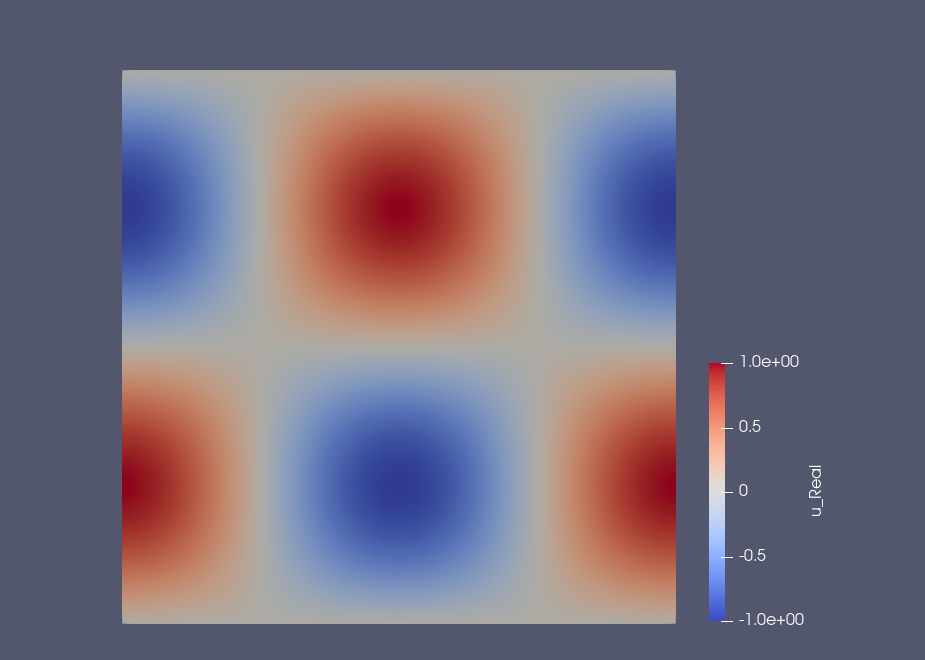
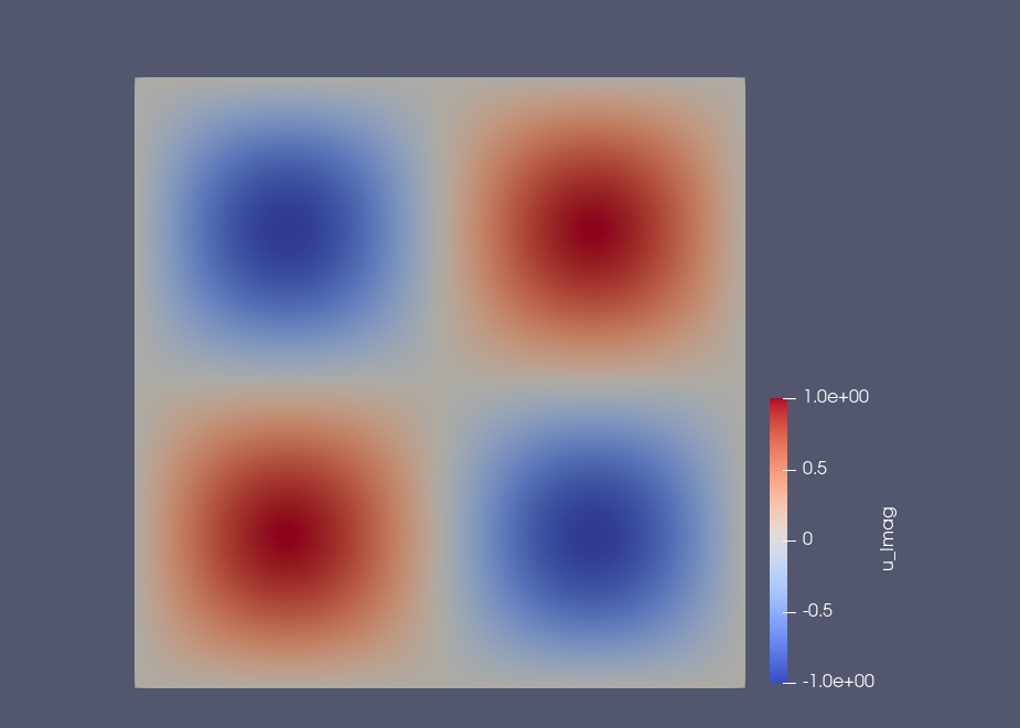
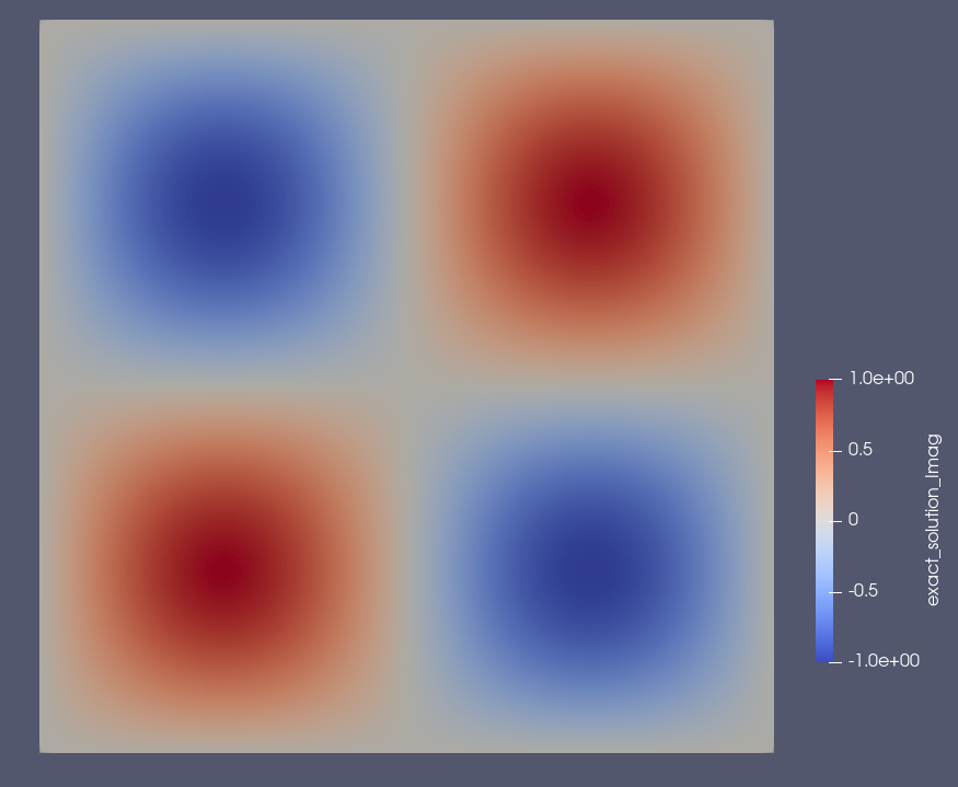
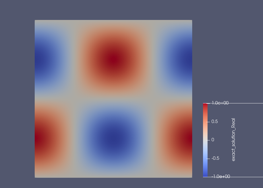
solution = exp(1j * kappa * x) * sin(kappa * y)
e_w_0 = sin(kappa * y) # value of incoming wave at x=0, forall y
dx_e_w_0 = 1j*kappa*sin(kappa * y) # derivative wrt. x of incoming wave at x=0, forall y

V   = ScalarFunctionSpace('V', Omega, kind=None)
V.codomain_type='complex'

u, v = elements_of(V, names='u, v')

error  = u - solution

expr   = dot(grad(u),grad(v)) - 2 * kappa ** 2 * u * v

#we impose an incoming wave from the left and absorbing boundary conditions at the right.
boundary_expr = - 1j * kappa * u * v
x_boundary = Union(Omega.get_boundary(axis=0, ext=-1), Omega.get_boundary(axis=0, ext=1))
boundary_source_expr = - dx_e_w_0 * v - 1j * kappa * e_w_0 * v

a = BilinearForm((u, v), integral(Omega, expr) + integral(x_boundary, boundary_expr))
l = LinearForm(v, integral(Omega.get_boundary(axis=0, ext=-1), boundary_source_expr))

equation = find(u, forall=v, lhs=a(u,v), rhs=l(v))

l2norm = Norm(error, Omega, kind='l2')
h1norm = Norm(error, Omega, kind='h1')

Step 3: Discretizing the domain, spaces and equations

# Discretize the geometry and equation
from psydac.api.discretization import discretize
from psydac.api.settings import PSYDAC_BACKENDS

# The backends are as follows and can all be run with OpenMP by setting backend['omp'] = True.
# For all but the Python backend, compilation flags can be accessed and changed using backend['flags'].
# - Python backend: Generate and runs python files. Accessed via PSYDAC_BACKENDS['python']
# - Pyccel GCC backend: Accessed via PSYDAC_BACKENDS['pyccel-gcc']
# - Pyccel Intel backend: Accessed via PSYDAC_BACKENDS['pyccel-intel']
# - Pyccel PGI backend: Accessed via PSYDAC_BACKENDS['pyccel-pgi']
# - Pyccel Numba backend: Accessed via PSYDAC_BACKENDS['numba']

backend = PSYDAC_BACKENDS['python']

# Uncomment to use OpenMp
# import os
# os.environ['OMP_NUM_THREADS'] = "4"
# backend['omp'] = True

ncells = [30, 30]
degree = [3, 3]
periodic = [False, True]

nquads = [p + 1 for p in degree]

# MPI version
# from mpi4py import MPI
# comm = MPI.COMM_WORLD
# Omega_h = discretize(Omega, ncells=ncells, comm=comm)
Omega_h = discretize(Omega, ncells=ncells, periodic=periodic)

Vh         = discretize(V, Omega_h, degree=degree)
equation_h = discretize(equation, Omega_h, [Vh, Vh], nquads=nquads, backend=backend)
l2norm_h   = discretize(l2norm, Omega_h, Vh, nquads=nquads, backend=backend)
h1norm_h   = discretize(h1norm, Omega_h, Vh, nquads=nquads, backend=backend)

Step 4: Solving the equation and computing the error norms

# Set the solver parameters
# 'cbig' -> Biconjugate gradient method
equation_h.set_solver('bicg', info=True, tol=1e-14)

import time

t0_s     = time.time()
uh, info = equation_h.solve()
t1_s     = time.time()


t0_d     = time.time()
l2_error = l2norm_h.assemble(u=uh)
h1_error = h1norm_h.assemble(u=uh)
t1_d     = time.time()

print( '> CG info       :: ',info )
print( '> L2 error      :: {:.2e}'.format(l2_error))
print( '> H1 error      :: {:.2e}'.format(h1_error))
print( '> Solution time :: {:.2e}s'.format(t1_s - t0_s))
print( '> Evaluat. time :: {:.2e}s '.format(t1_d - t0_d))

/opt/hostedtoolcache/Python/3.10.19/x64/lib/python3.10/site-packages/psydac/linalg/solvers.py:93: Warning: Solver 'bicg' currently not tested with complex operators.
  warnings.warn(msg, Warning)

> CG info       ::  {'niter': 45, 'success': True, 'res_norm': 9.329589911751023e-15}
> L2 error      :: 2.07e-07
> H1 error      :: 3.80e-05
> Solution time :: 7.52e+00s
> Evaluat. time :: 6.06e-01s

Step 5: Saving the results

# Save the results using OutputManager
from psydac.api.postprocessing import OutputManager
import os

os.makedirs('results_Helmholtz', exist_ok=True)

Om = OutputManager(
    f'results_Helmholtz/space_info_{Omega.name}',
    f'results_Helmholtz/field_info_{Omega.name}',
# MPI version
#   comm=comm,
)

Om.add_spaces(V=Vh)
Om.export_space_info()

Om.set_static()
Om.export_fields(u=uh)

Om.close()

Step 6: Exporting the results to VTK and visualizing them with Paraview

# Export the results to VTK using PostProcessManager
from psydac.api.postprocessing import PostProcessManager
from sympy import lambdify

Pm = PostProcessManager(
    domain=Omega,
    space_file=f'results_Helmholtz/space_info_{Omega.name}.yaml',
    fields_file=f'results_Helmholtz/field_info_{Omega.name}.h5',
# MPI version
#   comm=comm,
)

# The complex fields will be exported in two field: a real and an imaginary field
Pm.export_to_vtk(
    f'results_Helmholtz/visu_{Omega.name}',
    grid=None,
    npts_per_cell=3,
    fields='u',
    additional_physical_functions={'exact_solution': lambdify(Omega.coordinates, solution, modules='numpy')}
)

Pm.close()

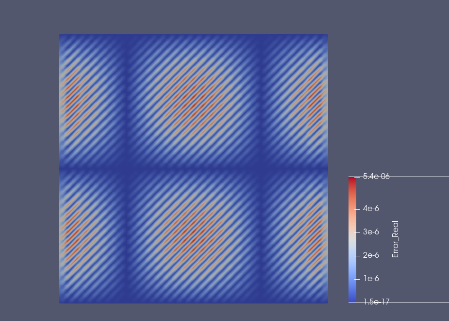
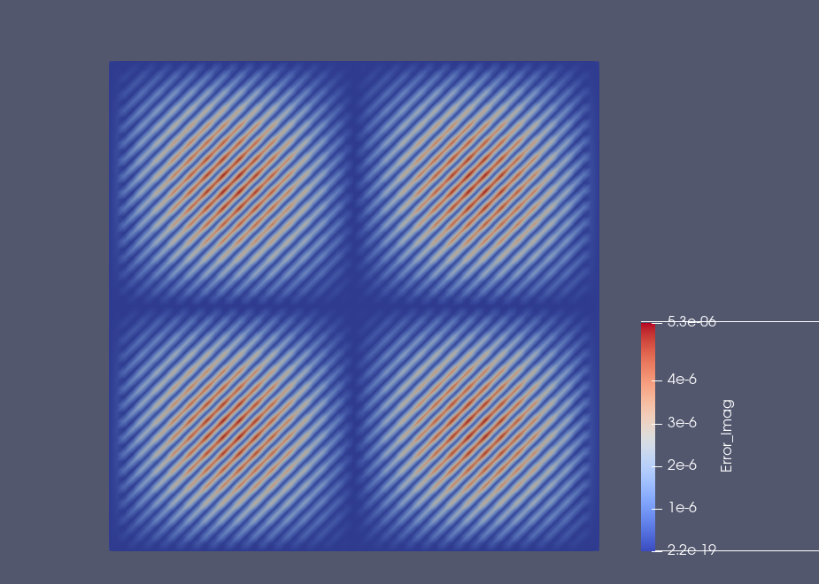
Example: Results on the square domain

Testing the notebook

import ipytest
ipytest.autoconfig(raise_on_error=True)

%%ipytest

def test_l2error():
    assert l2_error < 3e-07

def test_h1error():
    assert h1_error < 4e-05

..                                                                                           [100%]
2 passed in 0.02s