Computing the vector potential of a solenoidal field on a Torus#
A torus is a 3D domain with zero cavities and one tunnel.
As such, on a Torus, there exists only the trivial normal harmonic field, but a one-dimensional space of tangential harmonic fields.
Hence, any solenoidal field \(B\in H_0(div0)\) on a torus can be decomposed (Helmholtz decomposition) as
\(B = curl(A_0) + \lambda B_H\)
where \(B_H\) is a tangential harmonic field, and \(A_0\in H_0(curl)\) is the vector potential of the “harmonic-free” solenoidal field \(B - \lambda B_H\).
In this notebook, we compute a vector potential of the solenoidal magnetic field
\(B(x, y, z) = \left(\begin{matrix} (1/(x^2 + y^2)) \cdot ( (-C_0 y) + x(2z-1)(\sqrt{x^2 + y^2}-r)(\sqrt{x^2 + y^2}-R) ) \\ (1/(x^2 + y^2)) \cdot ( ( C_0 x) + y(2z-1)(\sqrt{x^2 + y^2}-r)(\sqrt{x^2 + y^2}-R) ) \\ (1/(x^2 + y^2)) \cdot ( \sqrt{x^2 + y^2}((r+R)-2\sqrt{x^2 + y^2})z(z-1) ) \end{matrix}\right),\quad\quad C_0=-10,\ r=0.5,\ R=1.\)
where \(r\) is the inner and \(R\) is the outer radius. We use this magnetic field as initial guess for a relaxation method for the computation of an MHD equilibrium.
We compute \(A_0\) and a vector potential of the tangential harmonic field \(B_H\) separately.
Step 1 : Computation of the “harmonic-free” vector potential \(A_0\)#
S.th. \(curl(A_0) = B - \lambda B_H\).
A (weak-divergence-free) vector potential \(A_0\in H_0(curl)\) of the “harmonic-free” part of \(B\) can be computed as the solution of the Hodge-Laplace problem
\(\left( \widetilde{curl}_h\ curl\ - grad\ \widetilde{div}_h \right) A_0 = \widetilde{curl}_h\ B.\)
Define and discretize the domain and the de Rham sequence#
[1]:
from    mpi4py  import MPI
import  numpy   as np

from    sympde.topology import Cube, Mapping, Derham

from    psydac.api.discretization import discretize

comm     = MPI.COMM_WORLD       # MPI communicator
ncells   = [16, 16, 16]         # number of cells in each direction
degree   = [3, 3, 3]            # B-spline degree in each direction
periodic = [False, True, False] # periodicity of the domain

r        = 0.5 # inner radius of the torus
R        = 1.  # outer radius of the torus

logical_domain = Cube('C', bounds1=(0.5,1), bounds2=(0,2*np.pi), bounds3=(0,1)) # 3D cubic domain - to be mapped to a toroidal domain (with square cross section)

class SquareTorus(Mapping):

    _expressions = {'x': 'x1 * cos(x2)',
                    'y': 'x1 * sin(x2)',
                    'z': 'x3'}

    _ldim        = 3
    _pdim        = 3

mapping = SquareTorus('ST')

domain   = mapping(logical_domain) # the mapped domain
derham   = Derham(domain)
domain_h = discretize(domain, ncells=ncells, periodic=periodic, comm=comm)
derham_h = discretize(derham, domain_h, degree=degree)

V0,   V1,   V2,   V3   = derham.spaces
V0h,  V1h,  V2h,  V3h  = derham_h.spaces
V0cs, V1cs, V2cs, V3cs = [Vh.coeff_space for Vh in derham_h.spaces]
Assembly of the system matrix#
corresponding to the bilinear form, and additionally taking care of homogeneous boundary conditions,
\(V^1_h\times V^1_h \ni (u, v) \mapsto \int curl(u)\cdot curl(v) + \widetilde{div}_h(u) \widetilde{div}_h(v)\)
[2]:
from    sympde.calculus         import inner
from    sympde.expr             import integral, BilinearForm
from    sympde.topology         import elements_of

from    psydac.api.settings     import PSYDAC_BACKEND_GPYCCEL
from    psydac.linalg.basic     import IdentityOperator
from    psydac.linalg.solvers   import inverse

backend = PSYDAC_BACKEND_GPYCCEL

G, C, D = derham_h.derivatives(kind='linop') # gradient, curl and divergence as psydac.linalg.basic.LinearOperator objects

# symbolic functions of the symbolic function spaces - to be used as trial and test functions
u0, v0 = elements_of(V0, names='u0, v0')
u1, v1 = elements_of(V1, names='u1, v1')
u2, v2 = elements_of(V2, names='u2, v2')
u3, v3 = elements_of(V3, names='u3, v3')

# Bilinear Forms corresponding to mass matrices of all four function spaces
m0 = BilinearForm((u0, v0), integral(domain, u0*v0))
m1 = BilinearForm((u1, v1), integral(domain, inner(u1, v1)))
m2 = BilinearForm((u2, v2), integral(domain, inner(u2, v2)))
m3 = BilinearForm((u3, v3), integral(domain, u3*v3))

# Discretization of the mass-matrix bilinear forms
m0h = discretize(m0, domain_h, (V0h, V0h), backend=backend)
m1h = discretize(m1, domain_h, (V1h, V1h), backend=backend)
m2h = discretize(m2, domain_h, (V2h, V2h), backend=backend)
m3h = discretize(m3, domain_h, (V3h, V3h), backend=backend)

# Assembly of the mass matrices
M0 = m0h.assemble()
M1 = m1h.assemble()
M2 = m2h.assemble()
M3 = m3h.assemble()

# Dirichlet projectors in order to apply the projection method
DP0, DP1, _, _ = derham_h.dirichlet_projectors(kind='linop')
I0             = IdentityOperator(V0cs)

# Modified mass matrix for the proper computation of the weak divergence
M0_0 = DP0 @ M0 @ DP0 + (I0 - DP0)

# Conjugate Gradient inverse of M0_0, preconditioned using an LST (Loli, Sangalli, Tani) preconditioner
M0_0_pc, = derham_h.LST_preconditioners(M0=M0, hom_bc=True)
M0_0_inv = inverse(M0_0, 'CG', pc=M0_0_pc, maxiter=1000, tol=1e-15)

# System matrix
S = C.T @ M2 @ C  +  M1 @ G @ M0_0_inv @ DP0 @ G.T @ M1
Assembly of the right-hand-side#
corresponding to the linear form
\(V^1_h \ni v \mapsto \int v\cdot\widetilde{curl}_h B\).
We also check whether
\(div(B) = 0\text{ in }\Omega\quad\quad\text{ and }\quad\quad n\cdot B=0\text{ on }\partial\Omega\)
hold.
[3]:
from    sympde.topology import Union, NormalVector

# Define callable function corresponding to B
def get_B(r, R, C0=-10):
    rad = lambda x, y : np.sqrt(x**2 + y**2)

    B1 = lambda x, y, z : (1/rad(x, y)**2) * ( (-C0 * y) + x * (2*z-1) * (rad(x, y)-r) * (rad(x, y)-R) )
    B2 = lambda x, y, z : (1/rad(x, y)**2) * ( ( C0 * x) + y * (2*z-1) * (rad(x, y)-r) * (rad(x, y)-R) )
    B3 = lambda x, y, z : (1/rad(x, y)**2) * (             rad(x, y) * ((r+R)-2*rad(x, y)) * z * (z-1) )

    B = (B1, B2, B3)
    return B

# Project B into V2h
_, _, P2, _ = derham_h.projectors()
r, R        = domain.logical_domain.bounds1

B           = P2(get_B(r, R))
b           = B.coeffs

# Check whether B is indead divergence free
div_b       = D @ b
div_b_norm  = np.sqrt( M3.dot_inner(div_b, div_b) )
print(f'||   div(B)   ||_L2(domain)  = {div_b_norm:.3g}')

# Check whether B is indead tangential to the boundary
def get_boundaries(*args):

    if not args:
        return ()
    else:
        assert all(1 <= a <= 6 for a in args)
        assert len(set(args)) == len(args)

    boundaries = {1: {'axis': 0, 'ext': -1},
                  2: {'axis': 0, 'ext':  1},
                  3: {'axis': 1, 'ext': -1},
                  4: {'axis': 1, 'ext':  1},
                  5: {'axis': 2, 'ext': -1},
                  6: {'axis': 2, 'ext':  1}}

    return tuple(boundaries[i] for i in args)

dir_zero_boundary = get_boundaries(1, 2, 5, 6) # we exclude the "periodic boundary" in y-direction as it is not technically a boundary anymore
boundary          = Union(*[domain.get_boundary(**kw) for kw in dir_zero_boundary])

# Assembly of "tangential trace mass matrix"
nn      = NormalVector('nn')
m2_bd   = BilinearForm((u2, v2), integral(boundary, inner(nn, u2) * inner(nn, v2)))
m2_bd_h = discretize(m2_bd, domain_h, (V2h, V2h), backend=backend, sum_factorization=False)
M2_bd   = m2_bd_h.assemble()

dirichlet_boundary_norm = np.sqrt( M2_bd.dot_inner(b, b) )
print(f'|| n \\cdot B ||_L2(boundary) = {dirichlet_boundary_norm:.3g}')

# Assembly of the right-hand-side
rhs = C.T @ M2 @ b
||   div(B)   ||_L2(domain)  = 3.59e-14
|| n \cdot B ||_L2(boundary) = 1.14e-15
Employ the projection method and solve for \(A_0\)#
[4]:
I1      = IdentityOperator(V1cs)

# Modify system matrix and right-hand-side in order to take care of boundary conditions
S_0     = DP1 @ S @ DP1 + (I1 - DP1)
rhs_0   = DP1 @ rhs

# Solve for A_0
maxiter = 1000
tol     = 1e-10

S_0_inv = inverse(S_0, 'cg', maxiter=maxiter, tol=tol)

a_0     = S_0_inv @ rhs_0
Step 2 : Computation of the vector potential \(A_H\) of \(B_H\)#
S.th. \(curl(A_H) = B_H\) and \(\|curl(A_H)\| = 1\).
The theoretical background for the computation of vector potentials of tangential harmonic fields has been recently published by Martin Campos Pinto and Julian Owezarek (https://arxiv.org/abs/2508.16822).
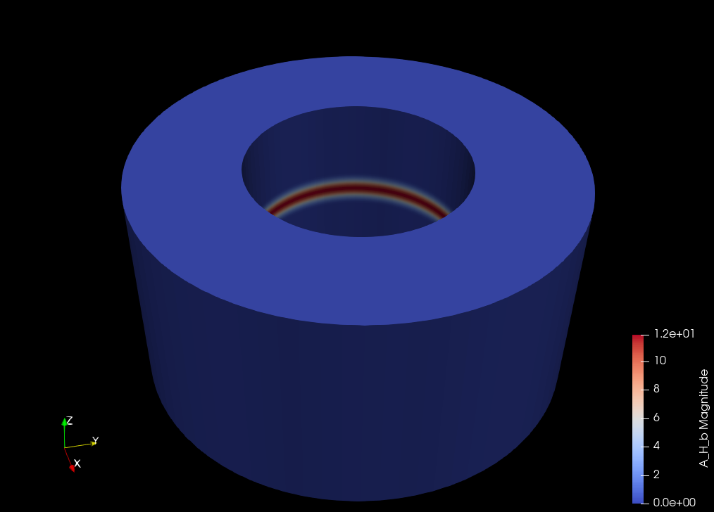
The potential is decomposed into \(A_H = A_H^b + A_H^0\). We call \(A_H^b\in H(curl)\) the lifting potential and \(A_H^0\in H_0(curl)\) the correction potential.
Construct a suitable choice of \(A^b_H\) for the torus#
[5]:
from    psydac.fem.basic        import FemField
from    psydac.linalg.utilities import array_to_psydac

def get_lifting_field():
    dim   = V1cs.dimension
    array = np.zeros(dim)

    nx, ny, nz = ncells
    px, py, pz = degree

    i3 = int(np.floor((nz+pz-1)/2))
    Nz = nz + pz

    start = (nx+px-1)*ny*(nz+pz) + (nx+px)*ny*(nz+pz)

    for i2 in range(ny):
        index = i2*(Nz-1) + i3
        array[start + index] = 1

    coeffs = array_to_psydac(array, V1cs)
    return coeffs

a_H_b = get_lifting_field()
Visualization of the lifting field#

Compute the correction potential \(A^0_H\)#
It’s yet again a solution to the previously introduced Hodge-Laplace problem, but now with a different right-hand-side
\(\left( \widetilde{curl}_h\ curl\ - grad\ \widetilde{div}_h \right) A^0_H = - \widetilde{curl}_h\ curl A^b_H.\)
[6]:
rhs_aH0   = - C.T @ M2 @ C @ a_H_b
rhs_aH0_0 = DP1 @ rhs_aH0

a_H_0 = S_0_inv @ rhs_aH0_0
Assemble the (normalized) harmonic potential \(A_H\) and compute \(\lambda\)#
s.th. \(B_H = curl(\lambda\ A_H)\)
[7]:
a_H = a_H_0 + a_H_b
a_H /= np.sqrt( M2.dot_inner(C @ a_H, C @ a_H) )

b_H = C @ a_H
lam = M2.dot_inner(b, b_H)
Step 3 : Assemble the entire vector potential and verify the solution#
\(A = A_0 + \lambda A_H\)
\(\epsilon := \| curl(A) - B \|_{L^2}\)
[8]:
a = a_0 + lam * a_H

diff   = C @ a - b
err_l2 = np.sqrt( M2.dot_inner(diff, diff) )
print(f'|| curl(A) - B ||_L2 = {err_l2:.3g}')
|| curl(A) - B ||_L2 = 4.79e-10
Step 4 : Save results#
[9]:
from    psydac.api.postprocessing import OutputManager
from    psydac.api.postprocessing import PostProcessManager
import  os

# B = curl(A_0) + curl(lam * A_H) =: B_0 + B_H = curl(A_0 + lam * A_H) =: curl(A)
B_H     = FemField(V2h,     C @ (lam * a_H))
B_0     = FemField(V2h, b - C @ (lam * a_H))
curlA   = FemField(V2h,     C @ a)

# A = A_0 + lam * A_H, here as above we write A_H and mean lam * A_H
A       = FemField(V1h,       a)
A_H     = FemField(V1h, lam * a_H)
A_0     = FemField(V1h,       a_0)

# lifting field A_H_b
A_H_b   = FemField(V1h, a_H_b)

# Save the results using OutputManager
# Export the results to VTK using PostProcessManager

os.makedirs('results_vector_potential', exist_ok=True)

Om = OutputManager(
    'results_vector_potential/space_info.yml',
    'results_vector_potential/field_info.h5',
    comm=comm,
    save_mpi_rank=True,
    mode = 'w'
)

Om.add_spaces(V1=V1h)
Om.add_spaces(V2=V2h)
Om.export_space_info()

Om.set_static() # the fields do not depend on time

save_fields = {
    'B'     : B,
    'B_H'   : B_H,
    'B_0'   : B_0,
    'curlA' : curlA,
    'A'     : A,
    'A_H'   : A_H,
    'A_0'   : A_0,
    'A_H_b' : A_H_b
}

Om.export_fields(**save_fields) # saves the coefficients of the fields

Om.close()

# This generates a YAML file containing the space information, and a HDF5 file that stores coefficients.
# At this point the solution has not been evaluated on any grid.

Pm = PostProcessManager(
    domain=domain,
    space_file=f'results_vector_potential/space_info.yml',
    fields_file=f'results_vector_potential/field_info.h5',
    comm=comm
)

Pm.export_to_vtk(
    f'results_vector_potential/visu',
    grid=None,
    npts_per_cell=[6,6,6],
    fields=save_fields.keys() # evaluate all the fields that were saved
)

Pm.close()
# If this file is run in sequential, then this step will generate a single .vtu file that can be opened with ParaView.
# If it is run in parallel, it generates a .vtu file per process (containing the local grid) and a .pvtu file. To visualize it in ParaView, open the .pvtu file.
Visualization in ParaView#
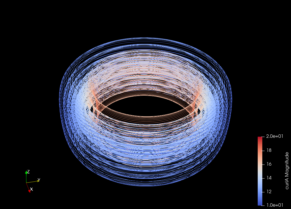
Compare \(B\) and \(curl(A)\)#

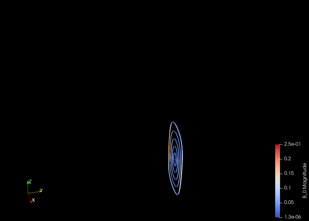
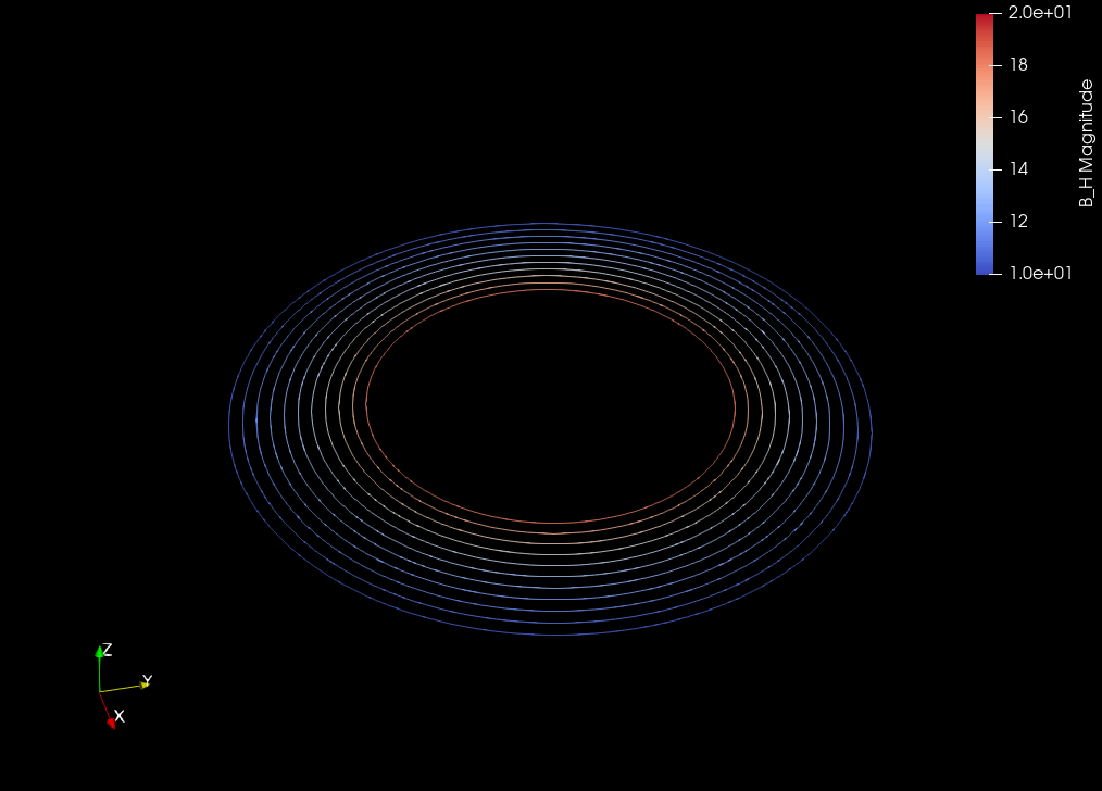
Inverstigate decomposition of \(B\) into \(B_0\), the harmonic-free part, and \(B_H\), the harmonic part#
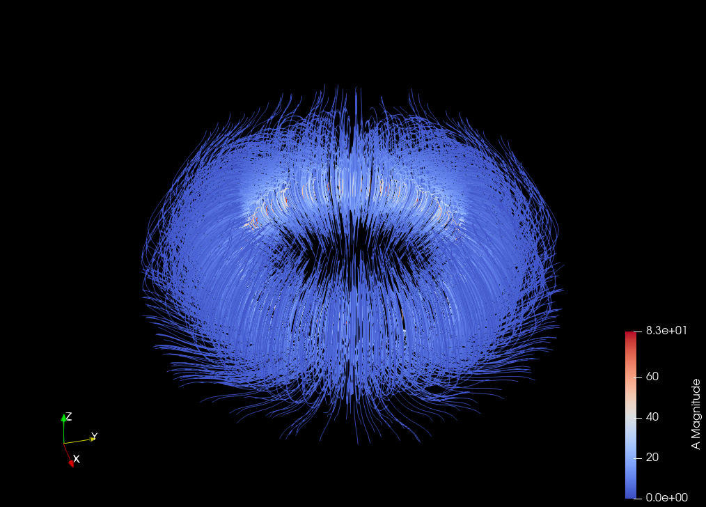
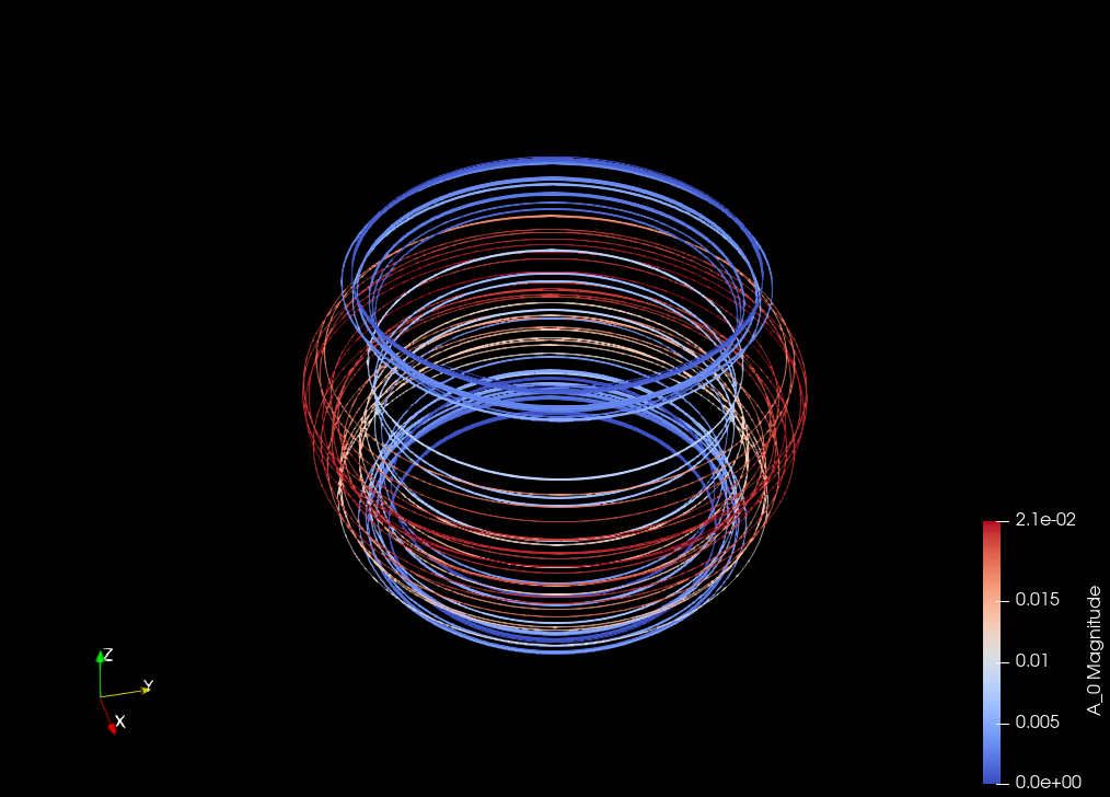
Invetsigate decomposition of \(A\) into \(A_0\), the potential of \(B_0\), and \(A_H\), the potential of \(B_H\)#