
Finite element projections of scalar and vector-valued functions#
Warning: this notebook is a draft, meant to discuss which interfaces should be exposed to users
In this notebook we show how to:
define FEM spaces over a given domain,
plot some FEM functions with a simple 2D plotting function,
apply H1 and Hcurl conforming projections to discrete multipatch fields,
assemble mass matrices and compute the L2 projections of some given functions.
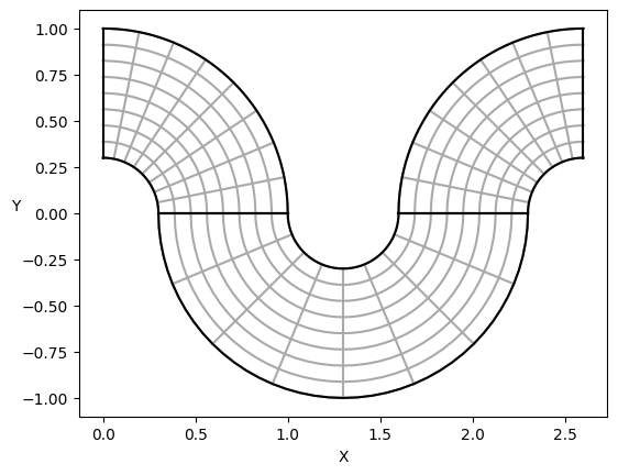
Step 1 : define a domain with sympde#
[1]:
import numpy as np
from sympde.topology import Square, PolarMapping

# Define each patch as a mapped subdomain
rmin, rmax = 0.3, 1.

domain_log_1 = Square('A_1', bounds1=(0., 1.), bounds2=(0., np.pi/2))
F_1 = PolarMapping('F_1', dim=2, c1=0., c2=0., rmin=rmin, rmax=rmax)
Omega_1 = F_1(domain_log_1)

domain_log_2 = Square('A_2', bounds1=(0., 1.), bounds2=(np.pi, 2 * np.pi))
F_2 = PolarMapping('F_2', dim=2, c1=rmin+rmax, c2=0., rmin=rmax, rmax=rmin)
Omega_2 = F_2(domain_log_2)

domain_log_3 = Square('A_3', bounds1=(0., 1.), bounds2=(np.pi/2, np.pi))
F_3 = PolarMapping('F_3', dim=2, c1=2*(rmin+rmax), c2=0., rmin=rmin, rmax=rmax)
Omega_3 = F_3(domain_log_3)

# Join the patches with the Domain.join function from sympde
from sympde import Domain
connectivity = [((Omega_1,1,-1), (Omega_2,1,-1), 1), ((Omega_2,1,1), (Omega_3,1,1), 1)]
patches = [Omega_1, Omega_2, Omega_3]
Omega = Domain.join(patches, connectivity, 'Omega')

# Simple visualization of the domain
from sympde.utilities.utils import plot_domain
npatches = len(Omega.subdomains)
print(f'A domain named {Omega}, with {npatches} patches:')
plot_domain(Omega, isolines=True)
A domain named Omega, with 3 patches:
Step 2 : define scalar and vector FEM spaces, plot some basis functions#
We first define a scalar-valued FEM space V
[2]:
from sympde.topology    import ScalarFunctionSpace, VectorFunctionSpace

# the kind argument specifies the pushforward defining the FEM space on the physical domain
# kind=None results in a space defined by a simple change of variable
V = ScalarFunctionSpace('V', Omega, kind=None)

ncells = [10, 10]
degree = [2, 2]

from psydac.api.discretization import discretize
Omega_h = discretize(Omega, ncells=ncells)
Vh = discretize(V, Omega_h, degree=degree)
print(f"we have defined a FEM space of type {type(Vh)}, with dimension {Vh.nbasis}")

# plot some basis function from the FEM space, using a simple wrapper for matplotlib
from psydac.fem.basic import FemField
from psydac.linalg.utilities import array_to_psydac

# here we set the coefficients by hand using numpy arrays
bf_c = np.zeros(Vh.nbasis)
i0 = 108
bf_c[i0] = 1
i1 = 211
bf_c[i1] = 1
i2 = 215
bf_c[i2] = 1
bf = FemField(Vh, coeffs=array_to_psydac(bf_c, Vh.coeff_space))

from psydac.fem.plotting_utilities import plot_field_2d
plot_field_2d(fem_field=bf, Vh=Vh, domain=Omega, cmap='viridis', title=fr'three scalar-valued basis functions: $\phi_{ {i0} }$, $\phi_{ {i1} }$, $\phi_{ {i2} }$', filename='')
we have defined a FEM space of type <class 'psydac.fem.vector.MultipatchFemSpace'>, with dimension 432
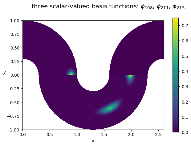
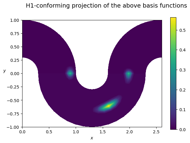
Note: the multipatch space Vh is made of discontinuous functions. A conforming projection may be used to map them to continuous functions
[3]:
from psydac.feec.conforming_projectors import construct_h1_conforming_projection
cP = construct_h1_conforming_projection(Vh, hom_bc=False)
Pbf = FemField(Vh, coeffs=array_to_psydac(cP@bf_c, Vh.coeff_space))
plot_field_2d(fem_field=Pbf, Vh=Vh, domain=Omega, cmap='viridis', title='H1-conforming projection of the above basis functions', filename='')
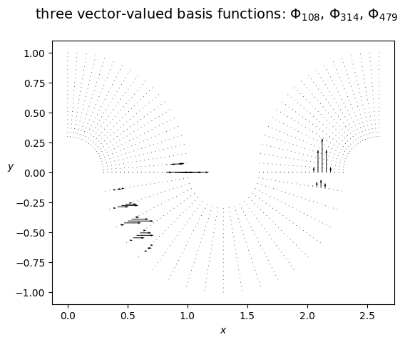
Then we define a vector-valued FEM space W
[4]:
# again, kind=None will result in a FEM space defined by a simple change of variable on the physical domain
W   = VectorFunctionSpace('W', Omega, kind=None)
Wh = discretize(W, Omega_h, degree=degree)
print(f"we have defined a FEM space of type {type(Wh)}, with dimension {Wh.nbasis}")

# plot some basis function from the space
# [remark] here I'm using numpy arrays, but one could illustrate the psydac indexing
dim_Wh = Wh.nbasis
bf2_c = np.zeros(dim_Wh)
i0 = 108; bf2_c[i0] = 1
i1 = 314; bf2_c[i1] = 1
i2 = 479; bf2_c[i2] = 1
bf2 = FemField(Wh, coeffs=array_to_psydac(bf2_c, Wh.coeff_space))

plot_field_2d(fem_field=bf2, Vh=Wh, domain=Omega,
    plot_type='components', cmap='viridis', title=fr'three vector-valued basis functions: $\Phi_{ {i0} }$, $\Phi_{ {i1} }$, $\Phi_{ {i2} }$', filename='')
we have defined a FEM space of type <class 'psydac.fem.vector.MultipatchFemSpace'>, with dimension 864
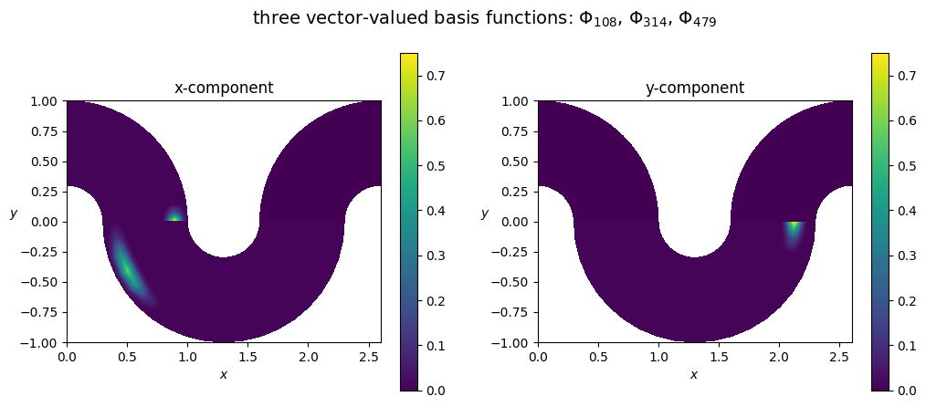
A stream plot of these basis functions is also possible, to better vizualise the vector fields
[5]:
plot_field_2d(fem_field=bf2, Vh=Wh, domain=Omega,
    plot_type='vector_field', vf_skip=1, title=fr'three vector-valued basis functions: $\Phi_{ {i0} }$, $\Phi_{ {i1} }$, $\Phi_{ {i2} }$', filename='')
Note: again, the multipatch space Wh is made of discontinuous functions. A conforming projection could be used, but continuity is harder to impose for vector-valued functions: this will be discussed in a further example.
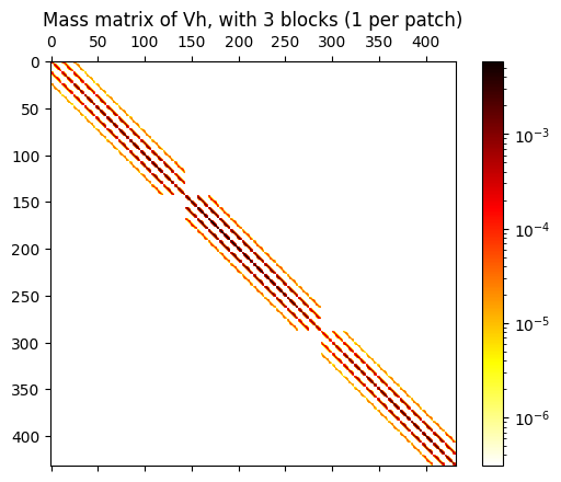
Step 3 : compute the mass matrices for Vh and Wh#
We assemble the mass matrices and visualize them. Again we start with the scalar-valued FEM space
[6]:
import matplotlib.pyplot as plt
from matplotlib import cm, colors

from sympde.topology    import elements_of
from sympde.expr.expr   import BilinearForm
from sympde.expr.expr   import integral

from psydac.api.settings import PSYDAC_BACKENDS

backend_language = 'python'

u, v = elements_of(V, names='u, v')
a = BilinearForm((u, v), integral(Omega, u * v))
ah = discretize(a, Omega_h, [Vh, Vh], backend=PSYDAC_BACKENDS[backend_language])

# Mass matrix in PSYDAC 'stencil' (linear operator) format
M_V = ah.assemble()

# visualize the mass matrix by plotting its numpy conversion
mat = M_V.toarray()
fig,ax = plt.subplots(1,1)
ax.set_title(f"Mass matrix of Vh, with {npatches} blocks (1 per patch)")
im = ax.matshow(mat, norm=colors.LogNorm(), cmap='hot_r')
cb = fig.colorbar(im, ax=ax)
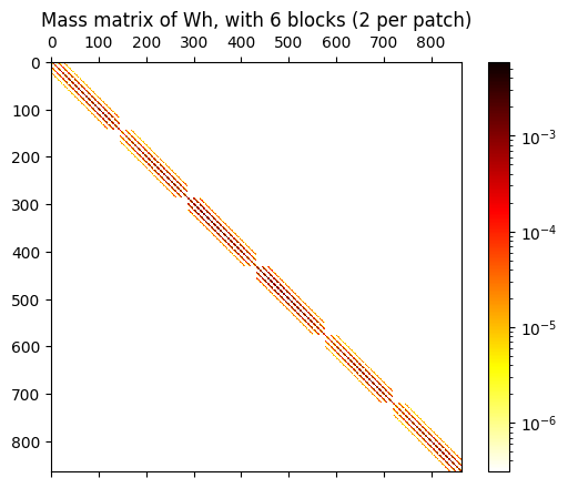
We next assemble the mass matrix of the vector-valued FEM space
[7]:
from sympde.calculus      import dot

uu, vv = elements_of(W, names='uu, vv')
a = BilinearForm((uu, vv), integral(Omega, dot(uu,vv)))
ah_W = discretize(a, Omega_h, [Wh, Wh], backend=PSYDAC_BACKENDS[backend_language])

# Mass matrix in PSYDAC 'stencil' (linear operator) format
M_W = ah_W.assemble()

# visualize the mass matrix by plotting its numpy conversion
mat_W = M_W.toarray()
fig,ax = plt.subplots(1,1)
ax.set_title(f"Mass matrix of Wh, with {2*npatches} blocks (2 per patch)")
im = ax.matshow(mat_W, norm=colors.LogNorm(), cmap='hot_r')
cb = fig.colorbar(im, ax=ax)
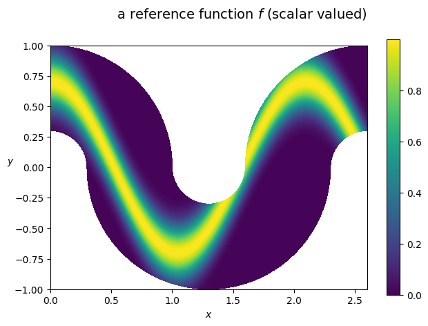
Step 4 : compute the moments of some given target function, and their L2 projections#
we first define a scalar function f and visualize it on the domain
[8]:
from sympy import cos, exp
x,y   = Omega.coordinates
ref_f = exp(-(y-0.7*cos(3*x))**2 / (2 * 0.15**2))

from sympy import lambdify
f_call = lambdify(Omega.coordinates, ref_f)  # make the expression a callable function

from psydac.fem.plotting_utilities import get_plotting_grid, my_small_plot
etas, xx, yy = get_plotting_grid(Omega.mappings, N=100)
ref_f_vals = [f_call(xx_k, yy_k) for xx_k, yy_k in zip(xx, yy)]

my_small_plot(
    title=r'a reference function $f$ (scalar valued)',
    vals=[ref_f_vals],
    xx=xx,
    yy=yy,
    save_fig='',
    cmap='viridis',
)
we next compute the moments of f in Vh and invert the mass matrix to get the L2 projection
[9]:
from psydac.linalg.solvers import inverse
from psydac.fem.projectors import get_dual_dofs

# the dual dofs are the moments, i.e. the products <f, phi_i>_{L2(Omega)}
tilde_f = get_dual_dofs(Vh=Vh, f=ref_f, domain_h=Omega_h, backend_language=backend_language)

inv_M = inverse(M_V, solver='cg')
f_coeffs = inv_M @ tilde_f
fh = FemField(Vh, f_coeffs)

plot_field_2d(fem_field=fh, domain=Omega, title=r'$f_h$: L2 projection of $f$ in Vh', cmap='viridis', filename='')

print('note the lower accuracy in the regions where the grid is not aligned with the anisotropic smoothness')
note the lower accuracy in the regions where the grid is not aligned with the anisotropic smoothness

compute the norm and the error
[10]:
from sympde.expr.expr          import Norm
error  = ref_f - u
err_l2norm = Norm(error, Omega, kind='l2')
nquads = [p + 1 for p in degree]
err_l2norm_h  = discretize(err_l2norm, Omega_h, Vh, nquads=nquads, backend=PSYDAC_BACKENDS[backend_language])
err_l2 = err_l2norm_h.assemble(u=fh)
print(f'> L2 projection error : {err_l2}')

zero_h = FemField(Vh, coeffs=array_to_psydac(np.zeros(Vh.nbasis), Vh.coeff_space))
f_l2 = err_l2norm_h.assemble(u=zero_h)
print(f'> L2 norm of f        : {f_l2}')

rel_err_f = err_l2 / f_l2
print(f'> L2 relative error   : {rel_err_f}')
> L2 projection error : 0.04758715258687875
> L2 norm of f        : 1.3385372111473266
> L2 relative error   : 0.035551609765177496
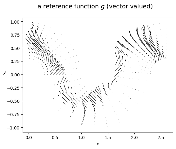
we then repeat the above steps for the vector-valued space Wh
[11]:
from sympy import pi, cos, Tuple

ref_g_x = ref_f * cos(2*pi*y)
ref_g_y = ref_f * 1
ref_g = Tuple(ref_g_x, ref_g_y)

# make the expression a callable function
g_vect = [lambdify(Omega.coordinates, ref_g[d]) for d in [0,1]]

ref_vals_g = [[g_vect[d](xx_k, yy_k) for xx_k, yy_k in zip(xx, yy)] for d in [0,1]]

from psydac.fem.plotting_utilities import my_small_streamplot
my_small_streamplot(
    title=r'a reference function $g$ (vector valued)',
    vals_x=ref_vals_g[0],
    vals_y=ref_vals_g[1],
    xx=xx,
    yy=yy,
    skip=8,
    amp_factor=1,
    hide_plot=False,
    dpi=200,
)
[12]:
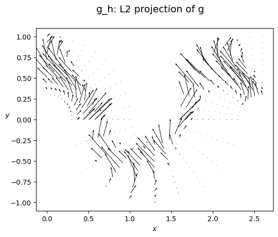
# again, the dual dofs are the moments relative to the basis of Wh, i.e. the products <g, Phi_i>_{L2(Omega)}
tilde_g = get_dual_dofs(Vh=Wh, f=ref_g, domain_h=Omega_h, backend_language=backend_language)

inv_M_W = inverse(M_W, solver='cg')
g_coeffs = inv_M_W @ tilde_g

gh = FemField(Wh, g_coeffs)

plot_field_2d(fem_field=gh, domain=Omega, plot_type='vector_field', title='g_h: L2 projection of g', filename='')
compute the norm and the error
[13]:
from sympy import Matrix

error = Matrix([ref_g[0]-uu[0], ref_g[1]-uu[1]])
err_l2norm = Norm(error, Omega, kind='l2')
nquads = [p + 1 for p in degree]
err_l2norm_h  = discretize(err_l2norm, Omega_h, Wh, nquads=nquads, backend=PSYDAC_BACKENDS[backend_language])
err_l2 = err_l2norm_h.assemble(uu=gh)
print(f'> L2 projection error : {err_l2}')

zero_h = FemField(Wh, coeffs=array_to_psydac(np.zeros(Wh.nbasis), Wh.coeff_space))
g_l2 = err_l2norm_h.assemble(uu=zero_h)
print(f'> L2 norm of g        : {g_l2}')

rel_err_g = err_l2 / g_l2
print(f'> L2 relative error   : {rel_err_g}')
> L2 projection error : 0.06370659279397187
> L2 norm of g        : 1.6364530376335813
> L2 relative error   : 0.03892967981904069
Testing the notebook#
[14]:
import ipytest
ipytest.autoconfig(raise_on_error=True)
[15]:
%%ipytest

def test_l2error_f():
    assert rel_err_f < 5e-02

def test_l2error_g():
    assert rel_err_g < 5e-02
..                                                                                           [100%]
2 passed in 0.02s