
Solving the time-harmonic Maxwells equations on a multipatch domain#
For \(\omega \in \mathbb{R}\) and \(\boldsymbol{J} \in L^2(\Omega)\), we solve
\[- \omega^2 \boldsymbol{E} + \mathbf{curl} \mathrm{curl} \boldsymbol{E} = \boldsymbol{J},\]
where \(\boldsymbol{E} \in H(\mathrm{curl}, \Omega).\)
Step 1: Discretize the domain.#
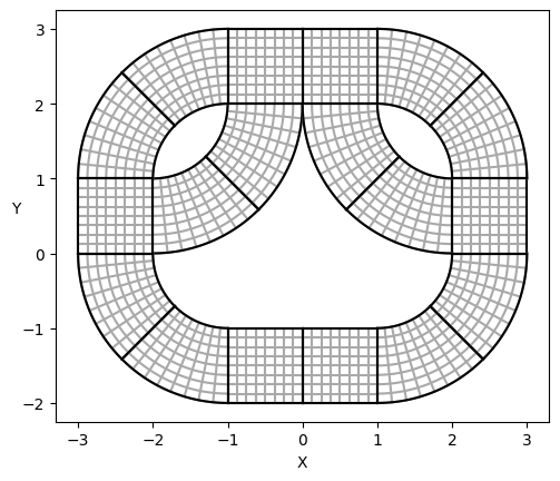
For the domain \(\Omega\), we choose the pretzel domain:
[1]:
from psydac.feec.multipatch_domain_utilities import build_multipatch_domain

domain = build_multipatch_domain(domain_name='pretzel_f')

from sympde.utilities.utils import plot_domain
plot_domain(domain, isolines=True)
Step 2: Discretize the de Rham sequence#
[2]:
from psydac.api.discretization import discretize
from sympde.topology import Derham

degree = [2, 2]
# For simplicity, we use the same number of cells for all patches
ncells = [4, 4]

derham = Derham(domain, ["H1", "Hcurl", "L2"])

domain_h = discretize(domain, ncells=ncells)
derham_h = discretize(derham, domain_h, degree=degree)
Step 3: Obtain the FEEC operators#
[3]:
# Finite Element spaces
V0h, V1h, V2h = derham_h.spaces

# Geometric global projectors
nquads = [(d + 1) for d in degree]
P0, P1, P2 = derham_h.projectors(nquads=nquads)

# Identity operator
from psydac.linalg.basic import IdentityOperator
I1 = IdentityOperator(V1h.coeff_space)

# Hodge and dual Hodge operators
H0, H1, H2 = derham_h.hodge_operators(kind='linop')
dH0, dH1, dH2 = derham_h.hodge_operators(kind='linop', dual=True)

# Conforming projectors with homogeneous boundary conditions
cP0, cP1, cP2 = derham_h.conforming_projectors(kind='linop', hom_bc=True)

# Broken derivative operators
bD0, bD1 = derham_h.derivatives(kind='linop')
Step 4: Assemble the system matrices#
[4]:
import numpy as np
omega = np.pi

CC = cP1.T @ bD1.T @ H2 @ bD1
M = -omega**2 * cP1.T @  H1
pre_A = M + CC

JS = 10 * (I1 - cP1).T @ H1 @ (I1 - cP1)

A =  pre_A @ cP1 + JS
Step 5: Source and exact solution#
[5]:
def get_source_and_solution_hcurl(eta=0, domain=None):
    from sympy import pi, cos, sin, Tuple, exp

    x, y = domain.coordinates

    # used for Maxwell equation with manufactured solution
    f_vect = Tuple(eta * sin(pi * y) - pi**2 * sin(pi * y) * cos(pi * x) + pi**2 * sin(pi * y),
                    eta * sin(pi * x) * cos(pi * y) + pi**2 * sin(pi * x) * cos(pi * y))

    u_ex = Tuple(sin(pi * y), sin(pi * x) * cos(pi * y))


    from sympy import lambdify
    u_ex_x = lambdify(domain.coordinates, u_ex[0])
    u_ex_y = lambdify(domain.coordinates, u_ex[1])

    return f_vect, [u_ex_x, u_ex_y]
Step 6: Get and project source#
[6]:
f_vect, u_ex = get_source_and_solution_hcurl(eta=-omega**2, domain=domain)

from psydac.fem.projectors  import get_dual_dofs
tilde_f = get_dual_dofs(Vh=V1h, f=f_vect, domain_h=domain_h)
f = dH1.dot(tilde_f)

# filtering the discrete source
tilde_f = cP1.T @ tilde_f
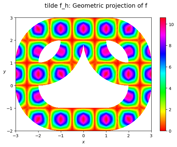
[7]:
from psydac.fem.plotting_utilities import plot_field_2d as plot_field
plot_field(stencil_coeffs=f, Vh=V1h, space_kind='hcurl', domain=domain, title='tilde f_h: Geometric projection of f', hide_plot=False)
saving contour plot in file dummy_plot.png
[8]:
# Manipulate the source to account for inhomogeneous boundary conditions in u
ubc = P1(u_ex).coeffs
ubc -= cP1 @ ubc

tilde_f -= pre_A @ ubc
Step 7: Solve the linear system using CG#
[9]:
from psydac.linalg.solvers     import inverse

solver = inverse(A, solver='cg', tol=1e-5)
u = solver.solve(tilde_f)
[10]:
# Project back to the full space and add the boundary conditions
u = cP1.dot(u)
u += ubc
Step 8: Look at the exact solution and compute the error#
[11]:
uex = P1(u_ex).coeffs
err = uex - u
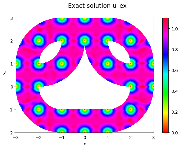
l2_error = np.sqrt(H1.dot_inner(err, err) / H1.dot_inner(uex, uex))
print('L2 relative error = ', l2_error)
L2 relative error = 0.007204955719418569
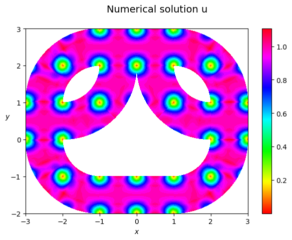
[12]:
plot_field(stencil_coeffs=u, Vh=V1h, space_kind='hcurl', domain=domain, title='Numerical solution u', hide_plot=False)
saving contour plot in file dummy_plot.png
[13]:
plot_field(stencil_coeffs=uex, Vh=V1h, space_kind='hcurl', domain=domain, title='Exact solution u_ex', hide_plot=False)
saving contour plot in file dummy_plot.png
Test the notebook#
[14]:
import ipytest
ipytest.autoconfig(raise_on_error=True)
[15]:
%%ipytest

def test_l2error():
    assert l2_error < 8e-03
.                                                                                            [100%]
1 passed in 0.01s