
Example of computing approximative eigenvalues with PETSc#
In this notebook we show how to compute approximative eigenvalues using PETSc. We use Conjugate Gradient to solve a 3D problem in parallel. Besides, we use a Jacobi preconditioner to illustrate how to set up a preconditioned Krylov solver with PETSc. The eigenvalues are estimated using the Krylov method and the number of estimated eigenvalues is the number of iterations.
Similar to the 3D VTK ParaView test, we solve the regularized curl curl problem in 3D with a callable function for the source. In practice, the source could be the interpolation of some experimental data. Besides, we impose periodic boundary conditions everywhere in the boundary.
Let \(\Omega=[0, 10] \times [-2\pi, 2\pi]\times [-3, 1]\). We want to find \(u\in H(\mathrm{curl}, \Omega)\) such that
where \(\mu = \pi\), and \(f\) is a callable function in terms of the domain coordinates, the expression of which is a priori not known.
Only for illustration here we use the callable function
and project it from \(H(\mathrm{curl}, \Omega)\) to the corresponding discretized space. This process is analogous with any callable vectorial function.
Step 1 : define the domain and spaces and discretize them#
This is similar to what is done in other examples
[1]:
import numpy as np
from mpi4py                     import MPI
from sympde.topology            import Cube
from sympde.topology            import VectorFunctionSpace
from psydac.api.discretization  import discretize

comm = MPI.COMM_WORLD # MPI communicator

Omega = Cube('Omega', bounds1=(0, 10), bounds2=(-2*np.pi, 2*np.pi), bounds3=(-3, 1)) # 3D cubic domain

W = VectorFunctionSpace('W', Omega, kind='hcurl') # Hcurl space

ncells = [25, 30, 11] # number of cells in each direction
degree = [3, 2, 2] # B-spline degree in each direction

periodic = [True, True, True] # set periodic BC in every direction

Omega_h = discretize(Omega, ncells=ncells, periodic=periodic, comm=comm)
Wh = discretize(W, Omega_h, degree=degree)
Step 2 : compute the matrix#
We assemble the mass and curl curl matrices.
[2]:
from sympde.topology      import elements_of, element_of
from sympde.expr.expr     import BilinearForm, LinearForm, integral
from sympde.calculus      import dot, curl
from psydac.api.settings  import PSYDAC_BACKENDS
from psydac.fem.basic     import FemField

backend_language = 'pyccel-gcc'
backend = PSYDAC_BACKENDS[backend_language]

u, v = elements_of(W, names='u, v') #trial and test functions

m = BilinearForm((u, v), integral(Omega, dot(u, v)))
mh = discretize(m, Omega_h, [Wh, Wh], backend=backend)
M = mh.assemble()  # Mass matrix

k = BilinearForm((u, v), integral(Omega, dot(curl(u), curl(v))))
kh = discretize(k, Omega_h, [Wh, Wh], backend=backend)
K = kh.assemble()  # Curl curl matrix

mu = 1e-1

A = K + mu*M # system matrix, positive-definite
Step 3 : compute the right-hand size#
We project a callable function to the vector space and use it to assemble the right-hand side of the system.
[3]:
from psydac.feec.global_geometric_projectors    import GlobalGeometricProjectorHcurl
f_callable = [lambda x, y, z: 10*np.exp(-0.5*(x-4)**2 - 1.5*z**2 - 1e-1*y**2),
              lambda x, y, z: 0,
              lambda x, y, z: np.cos(y)*np.sin(x*np.pi/5)]

proj_Wh = GlobalGeometricProjectorHcurl(Wh, nquads=[p+1 for p in degree]) # get Hcurl projector, nquads is the number of points for the Gauss quadrature.
fh = proj_Wh(f_callable) # project callable to field in Wh

f = element_of(W, name='f') # free variable for the FemField

l = LinearForm(v, integral(Omega, dot(f,v)))
lh = discretize(l, Omega_h, Wh, backend=backend)
rhs = lh.assemble(f=fh)  # assmble RHS, f is a free parameter
Step 4 : solve system with PETSc#
First we convert matrix to a PETSc.Mat object and the right-hand side to a PETSc.Vec object. Then we solve the system with conjugate gradient and Jacobi preconditioner. We also compute the approximative eigenvalues during the Krylov method.
[4]:
from petsc4py import PETSc
from psydac.linalg.utilities import petsc_to_psydac

Ap = A.topetsc()
rhsp = rhs.topetsc()

# initial solution
u = rhsp.copy()
u.zeroEntries() # set all entries to zero

iterative_solver = PETSc.KSP().create(comm=comm) # create Krylov solver object
iterative_solver.setType(PETSc.KSP.Type.CG)
iterative_solver.setOperators(A=Ap, P=Ap) # set operator and preconditioner
preconditioner = iterative_solver.getPC()
preconditioner.setType(PETSc.PC.Type.JACOBI) # set Jacobi preconditioner, i.e. diagonal of matrix Ap
preconditioner.setUp()

iterative_solver.setNormType(PETSc.KSP.NormType.UNPRECONDITIONED) #use unpreconditioned norm for convergence

iterative_solver.setComputeEigenvalues(True) # compute eigenvalues during Krylov solver
def callback(ksp, iter, rnorm):
    if ksp.getComm().Get_rank() == 0:
        print(f'Iter {iter} | res = {"{:.2e}".format(rnorm)}')

iterative_solver.setMonitor(callback) # set a callback function to print iteration and residual.
iterative_solver.setTolerances(atol=1e-5, rtol=1e-2, max_it=100)
iterative_solver.setInitialGuessNonzero(True) #if True it uses the solution vector as initial guess, otherwise it takes zero.

iterative_solver.solve(rhsp, u)

eigenvalues_approx = iterative_solver.computeEigenvalues() # the array size is the number of CG iterations

# convert the solution back to PSYDAC
u_psydac = petsc_to_psydac(u, Wh.coeff_space)
uh = FemField(Wh, coeffs=u_psydac)
Iter 0 | res = 6.89e+00
Iter 1 | res = 7.27e+00
Iter 2 | res = 9.02e+00
Iter 3 | res = 1.12e+01
Iter 4 | res = 9.66e+00
Iter 5 | res = 6.60e+00
Iter 6 | res = 4.95e+00
Iter 7 | res = 3.78e+00
Iter 8 | res = 4.05e+00
Iter 9 | res = 2.94e+00
Iter 10 | res = 1.81e+00
Iter 11 | res = 1.39e+00
Iter 12 | res = 1.33e+00
Iter 13 | res = 1.00e+00
Iter 14 | res = 6.34e-01
Iter 15 | res = 2.43e-01
Iter 16 | res = 1.70e-01
Iter 17 | res = 1.53e-01
Iter 18 | res = 2.19e-01
Iter 19 | res = 1.86e-01
Iter 20 | res = 2.28e-01
Iter 21 | res = 2.09e-01
Iter 22 | res = 1.82e-01
Iter 23 | res = 1.08e-01
Iter 24 | res = 5.62e-02
Step 5 : Plot approximative eigenvalues#
The eigenvalues computed with the Krylov method are only approximative. The number of computed “eigenvalues” is the number of iterations.
[5]:
import matplotlib.pyplot as plt

if comm is None or comm.Get_rank() == 0:
    fig,ax = plt.subplots(1,1)
    ax.set_title(f"Eigenvalues estimated with CG {iterative_solver.getIterationNumber()} iterations")
    im = ax.scatter(np.arange(eigenvalues_approx.size), eigenvalues_approx)
    plt.xlabel('index')
    plt.show()

if comm is not None:
    comm.Barrier()
/opt/hostedtoolcache/Python/3.10.20/x64/lib/python3.10/site-packages/matplotlib/cbook.py:1719: ComplexWarning: Casting complex values to real discards the imaginary part
  return math.isfinite(val)
/opt/hostedtoolcache/Python/3.10.20/x64/lib/python3.10/site-packages/matplotlib/collections.py:200: ComplexWarning: Casting complex values to real discards the imaginary part
  offsets = np.asanyarray(offsets, float)
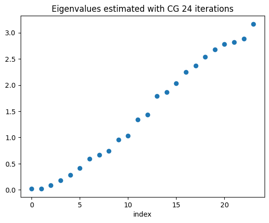
The estimated eigenvalues are shown above. We can see that the eigenavalues corresponding to the kernel of the curlcurl operator are shifted thanks to the regularization.
Step 6 : Save and export solution#
This step is similar to what is explained in other tests.
[6]:
# Save the results using OutputManager
from psydac.api.postprocessing import OutputManager
import os

os.makedirs('results_eigenvalues_regularized_curlcurl', exist_ok=True)

Om = OutputManager(
    f'results_eigenvalues_regularized_curlcurl/space_info_{Omega.name}.yml',
    f'results_eigenvalues_regularized_curlcurl/field_info_{Omega.name}.h5',
    comm=comm,
    save_mpi_rank=True,
    mode = 'w'
)

Om.add_spaces(V=Wh)
Om.export_space_info()

Om.set_static() # the fields do not depend on time

Om.export_fields(u=uh) # saves the coefficients of the solution

Om.close()

# Export the results to VTK using PostProcessManager
from psydac.api.postprocessing import PostProcessManager

Pm = PostProcessManager(
    domain=Omega,
    space_file=f'results_eigenvalues_regularized_curlcurl/space_info_{Omega.name}.yml',
    fields_file=f'results_eigenvalues_regularized_curlcurl/field_info_{Omega.name}.h5',
    comm=comm
)

Pm.export_to_vtk(
    f'results_eigenvalues_regularized_curlcurl/visu_{Omega.name}',
    grid=None,
    npts_per_cell=[4,2,4],
    fields='u'
)

Pm.close()