
Solving Poisson’s equation on a square domain with a mapped grid#
In this notebook, we will show how to solve Poisson’s equation on a single-patch square domain. Thanks to the simple geometry, will use the method of manufactured solution to build a test case where the exact solution is known a priori. As we are running this in a notebook, everything will be run in serial and hence we are limiting ourselves to a fairly coarse discretization to avoid taking too much time. However, PSYDAC allows for hybrid MPI + OpenMP parallelization with barely any changes to the code. The lines that are impacted by that will be preceeded by their MPI equivalent.
Step 1: Problem definition with SymPDE#
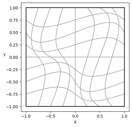
PSYDAC uses the powerful topological tools of SymPDE to build a large variety of domains. Here we use SymPDE to map a square domain \(\widehat{\Omega}\) to another square \(\Omega := F(\widehat{\Omega})\) with non-orthogonal coordinates. On such a simple domain, we define an exact solution \(u\) which satisfies homogeneous Dirichlet boundary conditions, and we compute the right-hand side \(f\) of the equation. The strong form of Poisson’s equation reads simply
[1]:
from sympy import sin, pi

from sympde.topology        import Square, CollelaMapping2D
from sympde.calculus        import laplace
from sympde.utilities.utils import plot_domain

# Problem definition
OmegaP = Square('Omega')                            # parametric domain
F      = CollelaMapping2D('F', eps=0.1, k1=1, k2=1) # mapping
Omega  = F(OmegaP)                                  # physical domain
x, y   = Omega.coordinates                          # physical coordinates
u_ex   = sin(pi * x) * sin(pi * y)                  # manufactured solution
f      = -laplace(u_ex)                             # right-hand side

# Simple visualization of the domain
plot_domain(Omega, isolines=True)
Step 2: Abstract weak formulation with SymPDE#
The weak formulation of Poisson’s equation reads:
Here \(H^1_0(\Omega)\) satisfies homogeneous Dirichlet boundary conditions. Currently, SymPDE does not allow attaching this information to the function space. (This is consistent with the fact that the FEM fields in PSYDAC are in general non-zero at the boundary.) Instead, an additional constraint is attached to the weak formulation explicitly, in the form of an EssentialBC object.
Since we are using the method of manufactured solutions, we can compute the \(L^2\) and \(H^1\) norms of the error. The norms are defined symbolically in SymPDE using Norm objects. The error is \(u-u_{ex}\), where the trial function \(u\) is a SymPDE ScalarFunction object, while the exact solution \(u_{ex}\) is a SymPy expression of the physical coordinates. Since \(u\) represents a free parameter, it will have to be replaced by a PSYDAC FEM field when assemblying
the norm.
[2]:
from sympde.topology import ScalarFunctionSpace
from sympde.topology import elements_of
from sympde.topology import NormalVector
from sympde.calculus import grad, inner
from sympde.expr     import LinearForm, BilinearForm, Norm
from sympde.expr     import integral
from sympde.expr     import find, EssentialBC

# Space, trial function u, and test function v
V    = ScalarFunctionSpace('V', Omega)
u, v = elements_of(V, names='u, v')

# Bilinear form a(u, v) and linear form l(v)
a  = BilinearForm((u, v),  integral(Omega, inner(grad(u), grad(v))))
l  = LinearForm(v, integral(Omega, f * v))

# Homogeneous Dirichlet boundary conditions: u=0 on ∂Ω
bc = EssentialBC(u, 0, Omega.boundary)

# Weak formulation of Poisson's eqn. with boundary conditions as constraint
equation = find(u, forall=v, lhs=a(u, v), rhs=l(v), bc=bc)

# L^2 and H^1 norms of the error
l2norm = Norm(u - u_ex, Omega, kind='l2')
h1norm = Norm(u - u_ex, Omega, kind='h1')
Step 3: Galerkin method with PSYDAC#
Starting from the weak formulation of Poisson’s equation, a Galerkin method of solution can be formulated as follows:
Let \(u_h \approx u\) in a finite dimensional subspace \(V_h \subset H^1_0\)
Choose a basis for \(V_h = span(\phi_1, \phi_2, \dots \phi_N)\)
Search for \(u_h(x,y) := \sum_{j=1}^N w_j\, \phi_j(x,y)\)
Choose test functions \(v = \phi_i\)
A linear PDE yields the linear system \(\mathbb{A}~\mathsf{w} = \mathsf{b}\)
PSYDAC provides the function discretize which maps SymPDE abstract objects to their discrete PSYDAC counterpart. For a Poisson problem over a single-patch domain, this means:
SymPDE |
PSYDAC |
|---|---|
|
|
|
|
|
|
|
|
|
|
|
|
In addition, SymPDE’s ScalarFunction objects correspond to PSYDAC’s FemField objects.
When discretizing an object of type Functional, LinearForm, or BilinearForm, PSYDAC automatically generates Python code for the corresponding assembly functions. This Python code can be accelerated to Fortran or C, and even include OpenMP instructions, depending on the “backend” chosen by the user. The available backends can be accessed through the PSYDAC_BACKENDS dictionary defined in the module psydac.api.settings, where the dictionary key is one the following strings:
['python', 'pyccel-gcc', 'pyccel-intel', 'pyccel-pgi', 'pyccel-nvidia']. Each of the dictionary values is itself a dictionary containing various options which can be modified by the user.
PSYDAC_BACKENDS['python'] defines a pure Python backend; this means that the generated Python assembly files will be used as they are. The other options are based on accelerating the Python assembly files using the Pyccel transpiler and one of the compilers: GCC, Intel, PGI, or NVIDIA. For all but the Python backend, OpenMP parallelization can be activated by setting backend['omp'] = True, and compilation flags can be accessed and changed using backend['flags'].
[3]:
from psydac.api.discretization import discretize
from psydac.api.settings import PSYDAC_BACKENDS

# Modify to use MPI and/or OpenMP
use_mpi    = False
use_openmp = False

# MPI communicator, if any
if use_mpi:
    from mpi4py import MPI
    comm = MPI.COMM_WORLD
else:
    comm = None

# Choose backend
backend = PSYDAC_BACKENDS['pyccel-gcc']
if use_openmp:
    import os
    os.environ['OMP_NUM_THREADS'] = "4"
    backend['omp'] = True

# Discretization parameters
ncells   = [9, 9]
degree   = [3, 3]
periodic = [False, False]
nquads   = [p + 1 for p in degree]

# Discretize domain and function space
Omega_h = discretize(Omega, ncells=ncells, periodic=periodic)
V_h     = discretize(V, Omega_h, degree=degree)

# Discretize weak formulation and error norms.
# Python code is generated for the assembly kernels.
# The number of quadrature points should be provided.
# If a Pyccel backend is chosen, the Python code is translated to Fortran.
equation_h = discretize(equation, Omega_h, [V_h, V_h], nquads=nquads, backend=backend)
l2norm_h   = discretize(l2norm, Omega_h, V_h, nquads=nquads, backend=backend)
h1norm_h   = discretize(h1norm, Omega_h, V_h, nquads=nquads, backend=backend)
Step 4: Solve the equation and compute the error norms#
When calling the assemble method of a DiscreteBilinearForm, DiscreteLinearForm, or DiscreteFunctional, PSYDAC assembles a matrix, vector, or scalar quantity, respectively. Objects of type DiscreteEquation do not have an assemble method, but they have the methods set_solver and solve instead:
The
set_solvermethod specifies the iterative algorithm (and its parameters) for solving the linear system \(\mathbb{A} \mathrm{w} = \mathrm{b}\) to obtain the spline coefficients \(\mathrm{w}\) of the Galerkin solution \(u_h\).The
solvemethods performs a few steps. First, it assembles both the left-hand-side matrix \(\mathbb{A}\) and right-hand-side vector \(\mathrm{b}\). Then, it solves the linear system \(\mathbb{A} \mathrm{w} = \mathrm{b}\) with the chosen iterative algorithm. Finally, it creates a callableFemFieldwith spline coefficients \(\mathrm{w}\).
[4]:
import time
from psydac.fem.plotting_utilities import plot_field_2d
# Set the solver parameters (CG = Conjugate Gradient)
equation_h.set_solver('CG', info=True, tol=1e-14)
# Compute the numerical solution u_h:
# 1. assemble (distributed) sparse matrix A
# 2. assemble (distributed) dense vector b
# 3. solve linear system A w = b
# 4. create callable field u_h(x,y)
t0_s = time.time()
u_h, info = equation_h.solve()
t1_s = time.time()
# Compute the L^2 and H^1 error norms
t0_d = time.time()
l2_error = l2norm_h.assemble(u=u_h)
h1_error = h1norm_h.assemble(u=u_h)
t1_d = time.time()
# Print convergence information, error norms, and timings
print('> CG info :: ',info )
print('> L2 error :: {:.2e}'.format(l2_error))
print('> H1 error :: {:.2e}'.format(h1_error))
print('> Solution time :: {:.2e} s'.format(t1_s - t0_s))
print('> Evaluat. time :: {:.2e} s'.format(t1_d - t0_d))
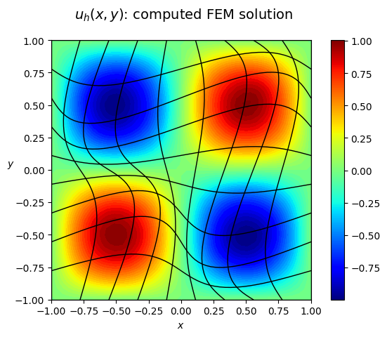
# Plot the results
plot_field_2d(u_h,
domain = Omega,
title = '$u_h(x,y)$: computed FEM solution',
plot_type = 'components',
N_vis = 50,
hide_plot = False,
filename = None,
cmap = 'jet',
)
> CG info       ::  {'niter': 60, 'success': True, 'res_norm': 7.78231042787227e-15}
> L2 error      :: 8.67e-03
> H1 error      :: 1.34e-01
> Solution time :: 2.30e-03 s
> Evaluat. time :: 2.16e-04 s
Testing the notebook#
[5]:
import ipytest
ipytest.autoconfig(raise_on_error=True)
[6]:
%%ipytest

def test_l2error():
    assert l2_error < 8.68e-03

def test_h1error():
    assert h1_error < 1.35e-01
..                                                                                           [100%]
2 passed in 0.14s